|
Climbing Mount Bourbaki
The following are the titles of recent articles syndicated from Climbing Mount Bourbaki
Add this feed to your friends list for news aggregation, or view this feed's syndication information.
LJ.Rossia.org makes no claim to the content supplied through this journal account. Articles are retrieved via a public feed supplied by the site for this purpose.
| Tuesday, November 19th, 2013 | | LJ.Rossia.org makes no claim to the content supplied through this journal account. Articles are retrieved via a public feed supplied by the site for this purpose. |
| 4:34 am |
Science, activism, and fossil fuel divestment Apologies for the long silence. It’s been a very hectic past few months, between working on multiple research projects and papers, applying to graduate schools, beginning a senior thesis, and increased involvement in Divest Harvard, where I’ve been coordinating the alumni wing of the campaign. I hope to have more to say about the first item in the next few weeks. In the meantime, here’s a talk that I gave that relates to the last.
I recently attended the 30th anniversary event of the Center for Excellence in Education, as an alum of the Research Science Institute, which was my first experience being a (however small) part of a mathematical community, and incidentally where I began blogging about mathematics. CEE offered attending alumni the chance to present short talks about topics of their choice. My talk, whose title is that of this post, is included below; the talk was also videotaped, and the video has been posted online. Here is the text.
It is great to be here. I was RSI ’09, and it was one of the best summers of my life. I would like to thank the Center for Excellence in Education for making that experience possible, and for organizing today’s very enjoyable events.
Like most of you here today, I am a scientist — or rather, a scientist-in-training. I am a scientist because I think discovering new things is stimulating and exciting. Yet I want to make the case that making discoveries is not enough for the world we live in — and that we have an ethical obligation to do more, to transcend the traditional scientific position of neutrality.
Much has been said about the ethics of science, ranging from physicists’ work on nuclear weapons to the treatment of animals. But the question we face today isn’t a question about the ethics of science itself: it’s a question about what happens when science speaks and yet no one listens. How can science make itself heard? And should it?
As you may surmise, I am referring to the climate crisis. Decades after scientists have understood the role of fossil fuels in the warming of our planet, the world’s annual carbon dioxide emissions continue their steady growth. I know everyone here has heard a lecture about polar bears at some point in their lives. I don’t wish to repeat that — because it’s too abstract, and it overlooks the absolutely fundamental human rights dimensions of the crisis. Climate change, simply put, threatens hundreds of millions of lives, and my generation’s future. I believe that it represents one of the critical issues that future generations will judge us on — just as we judge previous generations by their positions on civil rights, or on slavery.
My generation is obviously not the first to take climate change seriously. Many people have been valiantly fighting climate change for decades, developing cleaner energy technologies and lobbying our political system — some of you may be among them. But these efforts have been insufficient, and for a clear reason: powerful forces stand in the way. And foremost among those forces is the fossil fuel industry.
Why is that? According to the IPCC and others, the world has a “carbon budget,” comprising some 565 gigatons of carbon dioxide that can be burned to have a 80% chance of at most two degrees warming, the upper limit that the international community has set for global warming. This “carbon budget” leaves us with a limited time window, roughly thirty years at our present rate, in which to transition to a low-carbon future. It’s no secret that the world is not on track to make that transition. This is, in fact, a huge understatement. The proven reserves of the world’s fossil fuel companies amount to 2,795 gigatons. At this point, there is no expectation — in the markets or otherwise — that they won’t all be burned, leaving almost no chance for a stable future. It’s clear that no industry wants to have to write off the vast majority of their assets — which makes the motivations for fossil fuel industry’s well-documented campaigns to block climate change legislation all the more evident.
That’s why thousands of students at universities across the country, and across the world, have been calling on their schools to divest from fossil fuel companies — along with activists at numerous local governments and religious institutions. I’ve been proud to have been one of them, through the Divest Harvard campaign. Since last fall, we’ve been putting pressure on our administration to divest by cultivating a groundswell of support from students, faculty, and alumni. We’ve had considerable success: for example, in a referendum last fall, 72\% of Harvard undergraduates voted for a resolution calling for divestment from fossil fuels. Nationally, so far, seven universities have divested, along with several religious institutions and local governments. We don’t expect this to be an easy or quick victory, but then again, climate change is complicated.
What is divestment? Divestment is the removal of one’s investments from a particular firm or industry, often for ethical reasons. As a tool for social change, it has illustrious precedent. After pressure from students and faculty, numerous universities, notably UC Berkeley, divested from South Africa in the 1980s, in addition to pension funds and state governments. This has been credited with helping to end the apartheid regime.
All the same, many of you are probably wondering about the connection between divestment and stopping the climate crisis. It’s admittedly true that divestment itself is no substitute for better solar panels and better policies. Divestment is, instead a tool, to stigmatize an industry whose very business model necessitates catastrophic warming. And as a tool it has enormous promise. A recent Oxford University study showed that previous divestment campaigns, such as divestment from apartheid South Africa, were highly effective in bringing about necessary restrictive legislation. That report, moreover, found concluded that fossil fuel divestment is growing much faster than any of the previous campaigns analyzed.
There are many questions that have been raised, by people generally in support of action on climate change, on divestment. It is not, after all, the type of technique traditionally used by the environmental movement. Classical environmentalism has focused on individual responsibility and moral suasion. Important as that is, it suffers from a fatal flaw: there is no way putting on a sweater can bring about a political solution on climate change. And we really do need a political solution on the climate crisis. The challenge is, after all, to convince a hugely profitable industry to write off the majority of its assets.
The most common counterargument against divestment observes that we are all complicit in the world’s dependence on fossil fuels. Nonetheless, I believe that it is the fossil fuel industry that has made it impossible for us not to be complicit: it has prevented the political action that would allow us meaningful alternatives. Given the size of its reserves, this was only rational on their part.
But another common counterargument, which we often hear both from scientists and researchers and from university administrators, states a position of neutrality. Scientists and researchers, especially those who study climate change, are reluctant to do anything that might be seen as politicizing their work. After all, we’ve been told that it’s our goal to make the discoveries, not to legislate.
Money managers claim that endowments and pension funds should maintain a neutrality to best ensure returns.
The problem with that is that climate change is an existential threat. It is not a political issue, and wanting a stable future is not a special interest. There is no neutral ground for us, as scientists, and there is no neutral ground for institutions — like our universities — that will be directly affected by climate change.
My generation is not, obviously, the first to understand the seriousness of the climate crisis. But members of my generation, at least the ones I’ve talked to, have a certain urgency in confronting the climate crisis — an intensity matched, perhaps, by the seriousness of the problem. Members of my generation tend to see climate change as more than a technical fix to be solved with engineering wizardry, but instead as a profound ethical issue. Though we didn’t cause the problem, we are, after all, the ones who will inherit a warming planet. In calling for divestment, our hope is that we can bring about a world that decides to keep four-fifth’s of the fossil fuel reserves in the ground.
As scientists and scientists-in-training, I believe we have a special obligation to confront the climate crisis. But I do not believe neutral research and education, the role that we and our universities traditionally play, can suffice: all the solar energy research in the world cannot help if we elect to keep burning coal anyway. I believe that there is a place for grassroots social activism on this, in which we can play a role.
The chasm between political organizing and scientific research is often vast. But the example of James Hansen, among others, suggests that it may be bridged at the highest levels of both. I hope many of you will consider bridging it yourself, whether by telling your alma mater that you won’t donate until it divests or by writing a letter to your senator explaining why you support a carbon tax.
Like most of you, I went to RSI because I wanted to solve hard problems. This may be the hardest problem the world has ever seen. I hope we can work together on it. Thank you. Filed under: climate change Tagged: climate change, divestment, rsi   | | Wednesday, July 3rd, 2013 | | LJ.Rossia.org makes no claim to the content supplied through this journal account. Articles are retrieved via a public feed supplied by the site for this purpose. |
| 1:49 am |
27 lines on a cubic surface In the previous post, we introduced the Fano scheme of a subscheme of projective space, as the Hilbert scheme of planes of a certain dimension on that subscheme. In this post, I’d like to work out an explicit example, of the 27 lines on a smooth cubic surface in  ; as we’ll see, the Fano scheme is 27 reduced points, and the count can be made with a little calculation on the Grassmannian. Although the calculation is elementary, I found it worthwhile to work carefully through it, not only for its intrinsic interest but also as motivation for the study of intersection theory on moduli spaces in general. Once again, most of this material is from Eisenbud-Harris’s draft book 3264 and All That. ; as we’ll see, the Fano scheme is 27 reduced points, and the count can be made with a little calculation on the Grassmannian. Although the calculation is elementary, I found it worthwhile to work carefully through it, not only for its intrinsic interest but also as motivation for the study of intersection theory on moduli spaces in general. Once again, most of this material is from Eisenbud-Harris’s draft book 3264 and All That.
1. The normal bundle as self-intersection
Suppose  is a smooth surface, imbedded in some projective space, and consider the scheme is a smooth surface, imbedded in some projective space, and consider the scheme  of lines in of lines in  . .
Fix a line  in in  . In this case, the normal sheaf . In this case, the normal sheaf  is actually a vector bundle of normal vector fields, given by the adjunction formula is actually a vector bundle of normal vector fields, given by the adjunction formula
^{\vee} = \left(\mathcal{O}_S(-L)/\mathcal{O}_S(-2L)\right)^{\vee} = \mathcal{O}_L(L).")
In particular, is a line bundle on  and has a well-defined degree. This degree is in fact the self-intersection and has a well-defined degree. This degree is in fact the self-intersection  of , considered as a divisor on the smooth surface . of , considered as a divisor on the smooth surface .
To see this, let’s recall the definition of the intersection multiplicity on a smooth surface: to find , one needs to compute the Euler characteristic
,")
where the tensor product is taken in the derived sense. In other words, the “derived tensor product”  accounts for the fact that transversality fails. To compute this, we can use the resolution on , accounts for the fact that transversality fails. To compute this, we can use the resolution on ,
 \rightarrow \mathcal{O}_S \rightarrow \mathcal{O}_L \rightarrow 0,")
and tensor with  to get that the derived tensor product is represented by the two-term complex to get that the derived tensor product is represented by the two-term complex
 \rightarrow \mathcal{O}_L .")
It follows that the Euler characteristic is given by
 - \chi(N_{S/L}^{\vee}) = \deg N_{S/L},")
by Riemann-Roch. (This is not specific to lines in .)
Geometrically, the degree of the normal bundle on is a measure of its “positivity:” a greater degree indicates more sections, which in turn indicates that can be (at least infinitesimally) deformed to a greater degree. This in turn should correspond to the positivity of the intersection multiplicity: the statement  implies that cannot be deformed into general position. implies that cannot be deformed into general position.
2. Adjunction again
In general, we have one more piece of information about the self-intersection if we know the surface . Namely, we have the adjunction formula
 = K_S|_L \otimes \mathcal{O}_L(L),")
and, taking degrees, this implies that

where  is the divisor of the canonical line bundle on . is the divisor of the canonical line bundle on .
Suppose that  is a surface of degree is a surface of degree  , so that we can use adjunction again to conclude that , so that we can use adjunction again to conclude that  H}") for for }") the hyperplane class. In this case, since the hyperplane class. In this case, since  , we get , we get
 + L.L,")
so that  . As . As  , this suggests that the surface is less and less likely to contain lines, or at least that they will be extremely “rigid.” , this suggests that the surface is less and less likely to contain lines, or at least that they will be extremely “rigid.”
Another interpretation of this is that, once  , the Hilbert scheme of curves on is smooth at , and is a (reduced) point near : that is, more generally, the Fano scheme consists of reduced points. In fact, the negativity of the normal bundle ( , the Hilbert scheme of curves on is smooth at , and is a (reduced) point near : that is, more generally, the Fano scheme consists of reduced points. In fact, the negativity of the normal bundle ( = 0}") ) implies that there are no first-order deformations of , so that the tangent space of vanishes at . ) implies that there are no first-order deformations of , so that the tangent space of vanishes at .
In fact, a very general surface of degree  in in  contains only divisors of degrees dividing : the Picard group is generated by the hyperplane class contains only divisors of degrees dividing : the Picard group is generated by the hyperplane class }") , by a theorem of Noether and Lefschetz. (In higher dimensions, Grothendieck’s version of the Lefschetz hyperplane theorem implies that the Picard group of a smooth hypersurface is always generated by , but in dimension , by a theorem of Noether and Lefschetz. (In higher dimensions, Grothendieck’s version of the Lefschetz hyperplane theorem implies that the Picard group of a smooth hypersurface is always generated by , but in dimension  , one needs and “very general.”) , one needs and “very general.”)
3. Counting
Let be a smooth cubic surface, so that is the zero locus in of a section )}") . Our goal in this section is to analyze the scheme of lines on . In the previous section, we saw that is always reduced and finite: in fact, by the analysis there, any line . Our goal in this section is to analyze the scheme of lines on . In the previous section, we saw that is always reduced and finite: in fact, by the analysis there, any line  has self-intersection has self-intersection  . .
In the previous post, we saw another computationally useful expression for as a subscheme of the Grassmannian }") of lines in : is the zero locus in of a certain section of lines in : is the zero locus in of a certain section  of a certain four-dimensional vector bundle of a certain four-dimensional vector bundle  on . The vector bundle in question assigned to each line on . The vector bundle in question assigned to each line  the global sections the global sections
);")
that is, it assigned to the restriction of all the cubic polynomials in to . (As we saw, this vector bundle was well-defined and could be defined as a direct image.) Since  is a global section of is a global section of }") , it naturally defines a section of . , it naturally defines a section of .
The zero-locus, both set-theoretically and scheme-theoretically, of defines precisely the scheme of lines in . Now, the statement that is reduced amounts precisely to saying that the section of }") is transverse to the zero section: in other words, the number of points in the zero locus is precisely the top Chern class (Euler class) of , integrated over . So, to count the number of lines on , we need to compute is transverse to the zero section: in other words, the number of points in the zero locus is precisely the top Chern class (Euler class) of , integrated over . So, to count the number of lines on , we need to compute }") ! In particular, the answer we’ll get is independent of the smooth surface , and it’ll require a calculation on the Grassmannian. ! In particular, the answer we’ll get is independent of the smooth surface , and it’ll require a calculation on the Grassmannian.
4. The Grassmannian
The Grassmannian is a four-dimensional smooth variety (it is a quadric hypersurface in  ), and its cohomology or Chow ring has concrete generators given by the Schubert cycles. Fix a point ), and its cohomology or Chow ring has concrete generators given by the Schubert cycles. Fix a point  , a line , a line  , and a 2-plane , and a 2-plane  which are “general.” which are “general.”
Then one has a natural hypersurface in the Grassmannian given by

consisting of lines meeting  . (In fact, it is the intersection of the Grassmannian with a hyperplane under the Plücker embedding . (In fact, it is the intersection of the Grassmannian with a hyperplane under the Plücker embedding  \subset \mathbb{P}^5}") .) There are natural codimension two loci .) There are natural codimension two loci

and a codimension three subvariety

It is a basic fact that the Chow ring (or cohomology ring) of the Grassmannian is the free module on these four classes, together with the fundamental class and  . In other words . In other words
![\displaystyle H^*(\mathbb{G}(1, 3); \mathbb{Z}) = \mathbb{Z}\left\{1, \Sigma_{\ell}, \Sigma_p, \Sigma_H, \Sigma_{p, H}, [\ast]\right\},](http://s0.wp.com/latex.php?latex=%5Cdisplaystyle+H%5E%2A%28%5Cmathbb%7BG%7D%281%2C+3%29%3B+%5Cmathbb%7BZ%7D%29+%3D+%5Cmathbb%7BZ%7D%5Cleft%5C%7B1%2C+%5CSigma_%7B%5Cell%7D%2C+%5CSigma_p%2C+%5CSigma_H%2C+%5CSigma_%7Bp%2C+H%7D%2C+%5B%5Cast%5D%5Cright%5C%7D%2C+&bg=ffffff&fg=000000&s=0 "\displaystyle H^*(\mathbb{G}(1, 3); \mathbb{Z}) = \mathbb{Z}\left\{1, \Sigma_{\ell}, \Sigma_p, \Sigma_H, \Sigma_{p, H}, [\ast]\right\},")
where ![{[\ast]}](http://s0.wp.com/latex.php?latex=%7B%5B%5Cast%5D%7D&bg=ffffff&fg=000000&s=0 "{[\ast]}") is the fundamental class (i.e., the class of a point). Moreover, one can compute the ring structure by intersecting cycles in general position: for instance, clearly is the fundamental class (i.e., the class of a point). Moreover, one can compute the ring structure by intersecting cycles in general position: for instance, clearly

Similarly,
![\displaystyle \Sigma_p^2 = [\ast], \quad \Sigma_H^2 = [\ast], \quad \Sigma_p . \Sigma_H = 0,](http://s0.wp.com/latex.php?latex=%5Cdisplaystyle+%5CSigma_p%5E2+%3D+%5B%5Cast%5D%2C+%5Cquad+%5CSigma_H%5E2+%3D+%5B%5Cast%5D%2C+%5Cquad+%5CSigma_p+.+%5CSigma_H+%3D+0%2C+&bg=ffffff&fg=000000&s=0 "\displaystyle \Sigma_p^2 = [\ast], \quad \Sigma_H^2 = [\ast], \quad \Sigma_p . \Sigma_H = 0,")
because, for instance, the first intersection consists of lines passing through two general points  . The third intersection is zero if . The third intersection is zero if  . .
Less clearly,
")
Here is an informal argument for this. To compute  , we take lines , we take lines  in general position and compute the intersection of cycles in general position and compute the intersection of cycles  , which consists of lines that meet two general lines . However, instead of taking in “truly” general position, we take them simply distinct and meeting at a point , which consists of lines that meet two general lines . However, instead of taking in “truly” general position, we take them simply distinct and meeting at a point  ; then the intersection of cycles consists of lines that either pass through the intersection ; then the intersection of cycles consists of lines that either pass through the intersection  or through the plane that span. or through the plane that span.
More precisely, to show that  , one can use Poincaré duality: it suffices to compute the intersection of both sides with , one can use Poincaré duality: it suffices to compute the intersection of both sides with  and and  . Now . Now

both consist of single points by choosing two general lines and a general point or plane. For instance,  is represented by lines that pass through a point and through two general lines : that means the line has to be in the intersection of the planes spanned by is represented by lines that pass through a point and through two general lines : that means the line has to be in the intersection of the planes spanned by  and and  . .
Example 1 This calculation implies that
![\displaystyle \Sigma_{\ell}^4 = (\Sigma_p + \Sigma_H)^2 = 2[\ast],](http://s0.wp.com/latex.php?latex=%5Cdisplaystyle+%5CSigma_%7B%5Cell%7D%5E4+%3D+%28%5CSigma_p+%2B+%5CSigma_H%29%5E2+%3D+2%5B%5Cast%5D%2C+&bg=ffffff&fg=000000&s=0 "\displaystyle \Sigma_{\ell}^4 = (\Sigma_p + \Sigma_H)^2 = 2[\ast],")
or that there are two lines in passing through four general lines.
Let’s now see how the Chern classes of the two-dimensional tautological bundle on given by )}") look in this basis. By definition, a section of look in this basis. By definition, a section of )}") gives a section of whose zero locus is precisely the lines contained in a hyperplane: so gives a section of whose zero locus is precisely the lines contained in a hyperplane: so
 = \Sigma_H.")
Given two linearly independent elements of , defining two hyperplanes in , the degeneracy locus of the two induced sections of consist of lines on which the restrictions of the two hyperplanes intersect: that is, lines which meet the intersection of the two hyperplanes. So
 = \Sigma_{\ell}.")
Using this, we can compute }") (which is the vector bundle (which is the vector bundle )}") ) using the splitting principle. Namely, if we write formally for the “Chern roots” of the set ) using the splitting principle. Namely, if we write formally for the “Chern roots” of the set  , then the Chern roots of the symmetric cube are , then the Chern roots of the symmetric cube are  , so the Euler class is , so the Euler class is
(2t_1 + t_2) = 9 c_2( 2c_1^2 + c_2) ,")
by expressing in terms of the elementary symmetric polynomials. In our case, this means that
 = 9 \Sigma_H ( 2 \Sigma_{\ell}^2 + \Sigma_H) = 27,")
by the previous formulas, and we get the twenty-seven lines on a cubic surface, as desired. Filed under: algebraic geometry Tagged: 27 lines, Chern classes, cubic surface, Grassmannian, Schubert cells  | | Monday, July 1st, 2013 | | LJ.Rossia.org makes no claim to the content supplied through this journal account. Articles are retrieved via a public feed supplied by the site for this purpose. |
| 1:21 am |
Fano schemes Let  be a subvariety (or scheme). A natural question one might ask is whether be a subvariety (or scheme). A natural question one might ask is whether  contains lines, or more generally, planes contains lines, or more generally, planes  and, if so, what the family of such look like. For example, if and, if so, what the family of such look like. For example, if  is a nonsingular quadric surface, then is a nonsingular quadric surface, then  has two families of lines (or “rulings”) that sweep out ; this corresponds to the expression has two families of lines (or “rulings”) that sweep out ; this corresponds to the expression

imbedded in via the Segre embedding. For a nonsingular cubic surface in , it is a famous and classical result of Cayley and Salmon that there are twenty-seven lines. In this post and the next, I’d like to discuss this result and more generally the question of planes in hypersurfaces.
Most of this material is classical; I recently learned it from Eisenbud-Harris’s (very enjoyable) draft textbook 3264 and All That.
1. Varieties of planes
Let be a variety. There is a natural subset of the Grassmannian }") of of  -planes in -planes in  (i.e., (i.e.,  -dimensional subspaces of -dimensional subspaces of  ) that parametrizes those -planes which happen to be contained in . This is called the Fano variety. ) that parametrizes those -planes which happen to be contained in . This is called the Fano variety.
However, the Fano variety has a natural (and possibly nonreduced) subscheme structure that arises from its interpretation as the solution to a moduli problem, so perhaps it should be called a Fano scheme. The first observation is that the itself has a moduli interpretation: it is the Hilbert scheme of -dimensional subschemes of consisting of subschemes whose Hilbert polynomial is given by  ; such a subscheme is necessarily a linear subspace. ; such a subscheme is necessarily a linear subspace.
This suggests that we should think of the Fano scheme as a Hilbert scheme.
Definition 1 The Fano scheme  of is the subscheme of of is the subscheme of  parametrizing subschemes parametrizing subschemes  whose Hilbert polynomial is . whose Hilbert polynomial is .
In particular, is a union of components of the Hilbert scheme . The advantage of this picture is that one can apply deformation theory to understand the local structure of . In general, the tangent space to at a point parametrizing a subscheme  is given by is given by
 = H^0( Y, \hom(\mathcal{I}_Y/\mathcal{I}_Y^2, \mathcal{O}_Y)),")
corresponding to the intuition that a small deformation of a subscheme should be given by a family of normal vector fields on  . .
This means that we can understand the tangent space to the Fano scheme at a given subspace ; it’s
 = H^0(L , \hom(\mathcal{I}_L/\mathcal{I}_L^2, \mathcal{O}_L)),")
where  is the ideal cutting out . is the ideal cutting out .
We can also present the Fano scheme explicitly as a subscheme of the Grassmannian. Suppose is cut out by sections
);")
that is, the  are homogeneous polynomials whose vanishing cuts out . Then consists of -planes on which these polynomials restrict to zero. More precisely, on the line bundle , there is a tautological-dimensional vector bundle , which assigns to a -plane are homogeneous polynomials whose vanishing cuts out . Then consists of -planes on which these polynomials restrict to zero. More precisely, on the line bundle , there is a tautological-dimensional vector bundle , which assigns to a -plane  the global sections the global sections )}") ; equivalently, if ; equivalently, if
 \times \mathbb{P}^r,")
is the universal -plane (the “incidence correspondence”), then the tautological bundle can be described as
,")
which defines the vector bundle on described informally above. Now each defines a section of }") on , and the Fano scheme is the subscheme of cut out by the vanishing of the . In favorable situations, this means that we can use the theory of Chern classes to understand the cycle in represented by . on , and the Fano scheme is the subscheme of cut out by the vanishing of the . In favorable situations, this means that we can use the theory of Chern classes to understand the cycle in represented by .
2. Some dimension counting
In the case is a hypersurface of degree , the Fano scheme is the zero locus of a single section of the vector bundle  on (of dimension on (of dimension  ), which means that we should expect the following: ), which means that we should expect the following:
- is a subscheme of of codimension
 . .
- The class of in the Chow ring (or cohomology ring) of is given by the top Chern class of the vector bundle
 . .
While this need not be true (the section of the vector bundle need not be in “general position”), we can conclude the second point, with appropriate multiplicities, if the first statement holds. Using the (known) structure of the cohomology of the Grassmannian, this gives a very efficient way of solving enumerative questions related to .
For instance, if  , so has dimension , so has dimension  = 2(r-1)}") , we find that the expected dimension of the Fano scheme , we find that the expected dimension of the Fano scheme  of lines on is given by of lines on is given by

If is smooth and  , a conjecture of Debarre and de Jong states that the real dimension is always the above “expected dimension.” , a conjecture of Debarre and de Jong states that the real dimension is always the above “expected dimension.”
If is general, however, the question simplifies and we can directly say something by considering the universal example again. Instead of fixing one , the strategy is to consider all of them at once. Consider the Hilbert flag scheme }") of pairs of pairs

where is a -plane and is a hypersurface of degree . By definition, the scheme fibers both over the Grassmannian and the Hilbert scheme of degree hypersurfaces in (which is simply a  ). ).
By definition, the fibers of over the point corresponding to a hypersurface is the scheme that we are interested in. The clever trick here is to consider the fibers in the other direction, which are much simpler. The fiber of over the point in parametrizing a -plane is the subscheme of the Hilbert scheme  consisting of hypersurfaces containing . In other words, it is the projectivization of the kernel of the surjective map of vector bundles consisting of hypersurfaces containing . In other words, it is the projectivization of the kernel of the surjective map of vector bundles
) \rightarrow \mathrm{Sym}^d \mathcal{V} ,")
where the first vector bundle is the trivial one corresponding to the vector space of degree polynomials.
This means that is actually a projective bundle over the Grassmannian ; in particular, it is actually a smooth variety of dimension given by
 = \dim \mathbb{G}(k, r) + \dim H^0(\mathbb{P}^r, \mathcal{O}(d)) - \dim H^0( \mathbb{P}^k, \mathcal{O}(d)) - 1.")
For instance, when , this works out to be
 = 2(r-1) + \binom{d + r}{r} - (d+1) - 1,")
and this is mapping to a . It follows that:
Proposition 2 If the expected dimension  , then the general degree hypersurface in contains no lines. , then the general degree hypersurface in contains no lines.
My impression is that the presence of lines (and more generally, of rational curves of higher degree) on a smooth variety is considered a type of “positivity” constraint on : for instance, a spectacular theorem of Mori states that the failure of nefness of the canonical bundle (a weak form of positivity) implies that contains rational curves. Conversely, a theorem of Clemens states that general hypersurfaces of high degree  (which are “negative” in that the canonical bundle is ample) contain no rational curves at all. In higher degree, the variety gets more and more negative, more and more complicated, and should contain fewer comparatively simple objects such as lines. (which are “negative” in that the canonical bundle is ample) contain no rational curves at all. In higher degree, the variety gets more and more negative, more and more complicated, and should contain fewer comparatively simple objects such as lines.
Nonetheless, it is not true that negativity in this sense corresponds precisely to the differential-geometric notion of negative curvature. For instance, a smooth hypersurface in  has trivial fundamental group by the Lefschetz hyperplane theorem, implying (by the Cartan-Hadamard theorem) that it does not have a metric of negative curvature. has trivial fundamental group by the Lefschetz hyperplane theorem, implying (by the Cartan-Hadamard theorem) that it does not have a metric of negative curvature.
Filed under: algebraic geometry Tagged: Fano scheme, Hilbert scheme  | | Friday, June 28th, 2013 | | LJ.Rossia.org makes no claim to the content supplied through this journal account. Articles are retrieved via a public feed supplied by the site for this purpose. |
| 2:44 am |
Dual curves, bitangents, and jet bundles Let  be a smooth degree curve. Then there is a dual curve be a smooth degree curve. Then there is a dual curve
^*,")
which sends  , to the (projectivized) tangent line at , to the (projectivized) tangent line at  . Such lines live in the dual projective space . Such lines live in the dual projective space ^*}") of lines in of lines in  . We will denote the image by . We will denote the image by  ; it is another irreducible curve, birational to ; it is another irreducible curve, birational to  . .
This map is naturally of interest to us, because, for example, it lets us count bitangents. A bitangent to will correspond to a node of the image of the dual curve, or equivalently it will be a point in where the dual map ^*}") fails to be one-to-one. In fact, if is general, then fails to be one-to-one. In fact, if is general, then  will have only nodal and cuspidal singularities, and we we will be able to work out the degree of . By the genus formula, this will determine the number of nodes in and let us count bitangents. will have only nodal and cuspidal singularities, and we we will be able to work out the degree of . By the genus formula, this will determine the number of nodes in and let us count bitangents.
The purpose of this post is to describe this, and to discuss this map from the point of view of jet bundles, discussed in the previous post.
1. Jet bundles and the dual map
Let )}") be the first jet bundle of the hyperplane bundle be the first jet bundle of the hyperplane bundle }") : : )}") is a two-dimensional vector bundle on whose fibers over a point record not only sections of , but their “derivatives” at : in other words, 1-jets. To compute with , we can use the exact sequence is a two-dimensional vector bundle on whose fibers over a point record not only sections of , but their “derivatives” at : in other words, 1-jets. To compute with , we can use the exact sequence
 \rightarrow J_1( \mathcal{O}_C(1)) \rightarrow \mathcal{O}_C(1) \rightarrow 0, \ \ \ \ \ (1)")
where the last map sends a 1-jet to its “value.” Moreover, given a global section of , we have (by “Taylor expansion”) a global section of .
Recall from the previous post that we have a map
 \rightarrow 0,")
where the three global sections of the jet bundle }") come from the global sections of , as before. The kernel come from the global sections of , as before. The kernel  of this map is a one-dimensional subbundle of of this map is a one-dimensional subbundle of  whose fiber above a point is the tangent line. whose fiber above a point is the tangent line.
This gives a description of the dual curve: the dual curve is the map  corresponding to the line subbundle corresponding to the line subbundle  . In other words, we use the universal property of : a map into is equivalent to giving a line subbundle of . (One could equivalently use line quotients; it is here that the “duality” appears.) . In other words, we use the universal property of : a map into is equivalent to giving a line subbundle of . (One could equivalently use line quotients; it is here that the “duality” appears.)
Proposition 1 The dual curve map ^*}") has degree has degree  }") . .
Proof: The dual curve map (or Gauss map) ^*}") has the property that has the property that }") pulls back to the line bundle on , which was the kernel of the surjection pulls back to the line bundle on , which was the kernel of the surjection }") . It thus suffices to compute the degree of the first Chern class of , which is minus the first Chern class of . It thus suffices to compute the degree of the first Chern class of , which is minus the first Chern class of }") . .
To do so, observe that from the exact sequence (1), the degree of is
 + d = (2g_C - 2) + 2d = (d-1)(d-2) - 2 + 2d,")
using the genus formula. This implies the claim. 
2. General properties of the dual map
In the previous section, we gave a definition of the dual map ^*}") in terms of jet bundles, and showed that the map had degree in terms of jet bundles, and showed that the map had degree }") . However, that in itself doesn’t determine the degree of the image: we don’t know that the map is birational onto its image, let alone what the singularities of its image . However, that in itself doesn’t determine the degree of the image: we don’t know that the map is birational onto its image, let alone what the singularities of its image ^*}") might look like. might look like.
So we should start with the following result, which requires characteristic zero:
Proposition 2 The dual map is birational onto its image.
Equivalently, it suffices to show that the general tangent line to is not a bitangent.
Proof: Here is a rough geometric argument, which is based upon the result that the bidual of a smooth curve is again. (The dual is not necessarily smooth, but one can still define a Gauss map  away from the singular locus.) away from the singular locus.)
To define the tangent line to at a point , take a point  near , and consider the secant line near , and consider the secant line  : as : as  , this will approach the tangent line. Thus, to define the tangent line to at a point , this will approach the tangent line. Thus, to define the tangent line to at a point ^*}") , which is interpreted as a line , which is interpreted as a line  , take lines , take lines ^*}") near (which are in , so are tangent lines to at some point), and “draw the line through and near (which are in , so are tangent lines to at some point), and “draw the line through and  .” In .” In ^{**} = \mathbb{P}^2}") , that corresponds to intersecting . , that corresponds to intersecting .
So if was the projectivized tangent line  for , then will map to, in the bidual, the intersection of and for , then will map to, in the bidual, the intersection of and  for close to . As , this intersection tends to , so the bidual of is for close to . As , this intersection tends to , so the bidual of is  . .
This already tells us something: now that we know the degree of , it tells us that the intersection of with a general line in ^*}") consists of consists of }") points. This means that if points. This means that if  is a general point, there are tangent lines to that pass through . We could see this (assuming birationality but without using Chern classes) as follows: if is given by the degree polynomial equation is a general point, there are tangent lines to that pass through . We could see this (assuming birationality but without using Chern classes) as follows: if is given by the degree polynomial equation  = 0}") , then the line through , then the line through ![{p = [1: 0: 0]}](http://s0.wp.com/latex.php?latex=%7Bp+%3D+%5B1%3A+0%3A+0%5D%7D&bg=ffffff&fg=000000&s=0 "{p = [1: 0: 0]}") and a point is tangent to at and a point is tangent to at  if and only if if and only if
 = 0.")
In other words, the condition on that the tangent line through pass through is that a certain degree  polynomial vanish on . So the collection of such is the intersection of polynomial vanish on . So the collection of such is the intersection of  with with  , which by Bezout’s theorem gives . , which by Bezout’s theorem gives .
To understand the singularities of the dual curve, we use the following result, which is a local calculation that we omit.
Proposition 3 If is not a flex point, then the Gauss map is an immersion at . If is a flex but not a hyperflex, then the dual curve has an ordinary cusp at the image of .
3. The Plücker formulas
Let be a smooth curve. In the previous section, we showed that the dual , and stated that if was general (no hyperflexes), then was not too singular: it had only nodes and cusps, with the nodes occurring at bitangents and cusps at flex lines.
We know now that the degree of is , and that is birational to , so the normalization has genus  . In other words, is a plane curve of degree with . In other words, is a plane curve of degree with  nodes and nodes and  cusps, if has bitangents and cusps, if has bitangents and  flexes. It follows that we have the Plücker formula flexes. It follows that we have the Plücker formula
(d-2)}{2} = g(C) = g(C^*) = \frac{(d^2 - d - 1)(d^2 - d - 2)}{2} - b - f,")
because each node and each cusp reduces the genus of the normalization of a plane curve by one from the “expected” one.
However, in the previous post, we showed that for a general plane curve of degree ,
,")
so that this formula enables us to work out the number of bitangents.
For a plane quartic, we have  and the genus is three; the degree of the dual curve is and the genus is three; the degree of the dual curve is  , which gives , which gives

and we showed in the previous post that  , which gives , which gives  as desired. as desired.
Filed under: algebraic geometry Tagged: jet bundles, plane curves, Plucker formula  | | Wednesday, June 26th, 2013 | | LJ.Rossia.org makes no claim to the content supplied through this journal account. Articles are retrieved via a public feed supplied by the site for this purpose. |
| 4:16 pm |
Jet bundles and flexes Let be a smooth plane quartic, so that is a nonhyperelliptic genus 3 curve imbedded canonically. In the previous post, we saw that bitangent lines to were in natural bijection with effective theta characteristics on , or equivalently spin structures (or framings) of the underlying smooth manifold.
It is a classical fact that there are  bitangents on a smooth plane quartic. In other words, of the bitangents on a smooth plane quartic. In other words, of the  theta characteristics, exactly of them are effective. A bitangent here will mean a line theta characteristics, exactly of them are effective. A bitangent here will mean a line  such that the intersection such that the intersection  is a divisor of the form is a divisor of the form }") for for  points, not necessarily distinct. So a line intersecting in a single point (with contact necessarily to order four) is counted as a bitangent line. In this post, I’d like to discuss a proof of a closely related claim, that there are points, not necessarily distinct. So a line intersecting in a single point (with contact necessarily to order four) is counted as a bitangent line. In this post, I’d like to discuss a proof of a closely related claim, that there are  flex lines. This is a special case of the Plücker formulas, and this post will describe a couple of the relevant ideas. flex lines. This is a special case of the Plücker formulas, and this post will describe a couple of the relevant ideas.
1. Jet bundles on curves
Let be a smooth curve and on a line bundle. Then, given  , there is a -dimensional jet bundle , there is a -dimensional jet bundle  , which is a vector bundle on whose fiber over a point consists of , which is a vector bundle on whose fiber over a point consists of  -jets of at : equivalently, this is the vector bundle -jets of at : equivalently, this is the vector bundle
).")
To make this precise, one way is to use the identification of the symmetric power  with the Hilbert scheme of length subschemes of ; one has a natural map with the Hilbert scheme of length subschemes of ; one has a natural map
,")
which, in terms of the definition of the Hilbert scheme, is given by the subscheme of  which is the diagonal with multiplicity . Now, given which is the diagonal with multiplicity . Now, given }") , there is a -dimensional vector bundle , there is a -dimensional vector bundle  on which sends a divisor on which sends a divisor  of degree (which is what parametrizes) to the -dimensional vector space of degree (which is what parametrizes) to the -dimensional vector space
);")
more precisely, if we consider the universal subscheme  , then above vector bundle on is given by , then above vector bundle on is given by
,")
for  the projections from the projections from  on each factor. The above definition and discussion are valid only for curves, but the definition of the jet bundles can be extended to any smooth variety. on each factor. The above definition and discussion are valid only for curves, but the definition of the jet bundles can be extended to any smooth variety.
To compute with the jet bundle, we note that  has a natural filtration whose subquotients are given by the line bundles has a natural filtration whose subquotients are given by the line bundles /\mathcal{L}(-(m+1)p))}") . These line bundles are precisely . These line bundles are precisely  : for example, when : for example, when  and is trivial, the line bundle sends and is trivial, the line bundle sends
/\mathcal{O}(-2p),")
and this is precisely the definition of the cotangent bundle. In other words, from this filtration, we find that there are exact sequences of vector bundles on ,

While these need not be split, they do (inductively) determine the topological type of  , and enable (for instance) calculation of the Chern classes. , and enable (for instance) calculation of the Chern classes.
2. Flex lines
The construction of jet bundles plays a fundamental role in solving problems of contact order. As an application, let’s consider (informally) the problem of counting flex points on a general plane curve of a given degree . A flex line, by definition, is a line which meets with order of contact  at a point. at a point.
Let’s try to rephrase the above problem in the language of jet bundles. We have a line bundle , with  linearly independent sections linearly independent sections  , so that a line in is simply a linear combination of these (up to scaling). Now, given a line bundle on , so that a line in is simply a linear combination of these (up to scaling). Now, given a line bundle on  , a global section of certainly defines global sections of for each ; this operation associates to a global section its Taylor expansion (to some order ) at each point. , a global section of certainly defines global sections of for each ; this operation associates to a global section its Taylor expansion (to some order ) at each point.
The upshot of this is that we get a map of vector bundles
) \otimes \mathcal{O}_C \rightarrow J_3 \mathcal{O}(1),")
or equivalently, three global sections of }") : namely, it sends a global line on to the Taylor expansion up to order 3 at a given point . By definition, is a flex point precisely when there is a line intersecting to order : namely, it sends a global line on to the Taylor expansion up to order 3 at a given point . By definition, is a flex point precisely when there is a line intersecting to order  , which means that the line maps to zero in , which means that the line maps to zero in }") . .
In other words, we have a three-dimensional vector bundle on , and three global sections of ; we’d like to ask what the locus where they fail to be independent is: that is the locus of flex lines. In fact, that locus is precisely where the section  of of }") vanishes, and the number of points in the vanishing locus is the degree or first Chern class of . So, the number of points where fail to be independent in the fiber of the jet bundle vanishes, and the number of points in the vanishing locus is the degree or first Chern class of . So, the number of points where fail to be independent in the fiber of the jet bundle  is is
) = c_1( J_2 \mathcal{O}(1)).")
Topologically, one has
 \sim \mathcal{O}_C(1) \oplus( K_C \otimes \mathcal{O}_C(1)) \oplus (K_C^{2} \otimes \mathcal{O}_C(1)),")
although this need not be true algebraically: the above is true only in the setting of topological bundles, or (better) in the Grothendieck group of algebraic vector bundles. However, using the adjunction relation
,")
we now find that (even as algebraic line bundles),
 \simeq \mathcal{O}_C(3 + 3(d-3) ),")
so that the degree of this line bundle on , or the number of flex points, is
.")
Taking  , we get the classical nine flex points on a smooth cubic: these correspond to the 3-torsion points of an elliptic curve under the usual imbedding. (This shows that, for an abstract plane cubic , while there is not necessarily a canonical basepoint to make into an elliptic curve, there is a natural space of nine possible choices, corresponding to the flex points.) For , the formula gives flexes on a smooth quartic curve. , we get the classical nine flex points on a smooth cubic: these correspond to the 3-torsion points of an elliptic curve under the usual imbedding. (This shows that, for an abstract plane cubic , while there is not necessarily a canonical basepoint to make into an elliptic curve, there is a natural space of nine possible choices, corresponding to the flex points.) For , the formula gives flexes on a smooth quartic curve.
In the above informal argument, there is a serious ignored issue of multiplicities. The argument was that the three-dimensional space of linear forms gave a canonical element of , which vanished precisely at the flexes. However, we didn’t count the multiplicities. A more detailed local analysis with jet bundles would show that at a hyperflex, where there is a line of order of contact  , the multiplicity of the vanishing of the section of is greater than one. In other words, the result is: , the multiplicity of the vanishing of the section of is greater than one. In other words, the result is:
Theorem 1 If is a smooth curve of degree with no hyperflexes, then has }") flex points. flex points.
To make this theorem non-vacuous, we should claim that the general degree  curve has no hyperflexes. To see this, let be the space of degree smooth curves (an open subset in a projective space). We consider the collection of triples curve has no hyperflexes. To see this, let be the space of degree smooth curves (an open subset in a projective space). We consider the collection of triples }") where: where:
- is a degree curve.
- is a point along the line .
This is flat over with fibers given by a flag variety, so has dimension  . Now consider the subvariety . Now consider the subvariety  where we require that , which cuts down the dimension by 1; so where we require that , which cuts down the dimension by 1; so  . But that’s not quite we want. Impose the stronger condition that . But that’s not quite we want. Impose the stronger condition that  has length at least four, to get a subvariety has length at least four, to get a subvariety  . To compute the dimension of . To compute the dimension of  , map to the flag variety, so that the fiber of above , map to the flag variety, so that the fiber of above }") consists of degree curves that meet at with contact to order . That is four linear conditions, so that consists of degree curves that meet at with contact to order . That is four linear conditions, so that  . In particular, the image of . In particular, the image of  is a proper subvariety; that’s equivalent to saying that most degree curves have no hyperflexes. is a proper subvariety; that’s equivalent to saying that most degree curves have no hyperflexes.
These ideas can be extended considerably (even for curves); for instance, they can be used to study the notion of ramification of a linear series, and thus count objects such as Weierstrass points. Filed under: algebraic geometry Tagged: flex lines, jet bundles  | | Monday, June 24th, 2013 | | LJ.Rossia.org makes no claim to the content supplied through this journal account. Articles are retrieved via a public feed supplied by the site for this purpose. |
| 4:20 am |
Theta characteristics and framings Let be an algebraic curve over  . A theta characteristic on is a (holomorphic or algebraic) square root of the canonical line bundle . A theta characteristic on is a (holomorphic or algebraic) square root of the canonical line bundle  , i.e. a line bundle , i.e. a line bundle }") such that such that

Since the degree of is even, such theta characteristics exist, and in fact form a torsor over the 2-torsion in the Jacobian  = \mathrm{Pic}^0(C)}") , which is isomorphic to , which is isomorphic to  \simeq (\mathbb{Z}/2\mathbb{Z})^{2g}}") . .
One piece of geometric motivation for theta characteristics comes from the following observation: theta characteristics form an algebro-geometric approach to framings. By a theorem of Atiyah, holomorphic square roots of the canonical bundle on a compact complex manifold are equivalent to spin structures. In complex dimension one, a choice of a spin structure is equivalent to a framing of  . On a framed manifolds, there is a canonical choice of quadratic refinement on the middle-dimensional mod homology (with its intersection pairing), which gives an important invariant of the framed manifold known as the Kervaire invariant. (See for instance this post on the paper of Kervaire that introduced it.) . On a framed manifolds, there is a canonical choice of quadratic refinement on the middle-dimensional mod homology (with its intersection pairing), which gives an important invariant of the framed manifold known as the Kervaire invariant. (See for instance this post on the paper of Kervaire that introduced it.)
It turns out that the mod function }") on the theta characteristics is precisely this invariant. In other words, theta characteristics give a purely algebraic (valid in all characteristics, at least on the theta characteristics is precisely this invariant. In other words, theta characteristics give a purely algebraic (valid in all characteristics, at least  ) approach to the Kervaire invariant, for surfaces! ) approach to the Kervaire invariant, for surfaces!
Most of the material in this post is from two papers: Atiyah’s Riemann surfaces and spin structures and Mumford’s Theta characteristics of an algebraic curve.
1. Examples
In genus two, every curve is hyperelliptic via the canonical map

which is ramified at six points  . The canonical divisor has the property that . The canonical divisor has the property that
, \quad 1 \leq i \leq 6,")
so that the line bundles }") (which are pairwise linearly inequivalent) give six theta characteristics. (which are pairwise linearly inequivalent) give six theta characteristics.
Since the theta characteristics form a torsor over the 2-torsion in the Jacobian, which is isomorphic to ^{4}}") , we should expect ten more theta characteristics. These will not be effective; for distinct , we should expect ten more theta characteristics. These will not be effective; for distinct  with with  , the line bundle corresponding to the divisor , the line bundle corresponding to the divisor

is a theta characteristic. (In fact,  is a 2-torsion point in the Jacobian, and as , these range over all the 15 nonzero 2-torsion points.) These form a (redundant) list of all the theta characteristics on . is a 2-torsion point in the Jacobian, and as , these range over all the 15 nonzero 2-torsion points.) These form a (redundant) list of all the theta characteristics on .
In genus three, given a theta characteristic , we observe that has degree two, so }") has dimension either has dimension either  , and the last one occurs only if is hyperelliptic. So suppose is a nonhyperelliptic genus three curve, which means that the canonical map , and the last one occurs only if is hyperelliptic. So suppose is a nonhyperelliptic genus three curve, which means that the canonical map
),")
imbeds as a smooth quartic in . In this case, there are the effective theta characteristics, each of which necessarily corresponds to a unique effective divisor  . To say that is a theta characteristic is to say that . To say that is a theta characteristic is to say that
 \simeq K \simeq \mathcal{O}(1),")
under the canonical imbedding: that is, the intersection of with a line in must cut out the subscheme  . This means that the line is necessarily tangent to at both . This means that the line is necessarily tangent to at both  , or in other words: , or in other words:
Proposition 1 Effective theta characteristics on the nonhyperelliptic genus three curve are in bijection with bitangent lines on .
In fact, counting theta characteristics can be used to prove a fact from enumerative geometry, that a smooth plane quartic has exactly bitangents.
2. Spin structures and theta
The purpose of this section is to describe the following interpretation of theta characteristics in geometry:
Theorem 2 (Atiyah) On a compact complex manifold , spin structures are in natural bijection with holomorphic square roots of the canonical bundle.
Proof: The holomorphic tangent bundle  is a complex vector bundle whose underlying is a complex vector bundle whose underlying  -bundle is isomorphic to the usual real tangent bundle of . In particular, it is a -bundle is isomorphic to the usual real tangent bundle of . In particular, it is a }") -bundle, and a spin structure consists of a lift of the underlying -bundle, and a spin structure consists of a lift of the underlying }") -bundle, under the map -bundle, under the map
 \rightarrow SO(2n),")
to a }") -bundle under the double covering map -bundle under the double covering map  \rightarrow SO(2n)}") ; equivalently, it is a lift in the diagram ; equivalently, it is a lift in the diagram
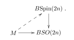
The choice of lifts to }") together with a homotopy to make the diagram commute) is canonically a together with a homotopy to make the diagram commute) is canonically a }") -torsor. Since pulls back to the unique two-fold cover -torsor. Since pulls back to the unique two-fold cover }") of , to give a spin structure on is equivalent to giving the tangent bundle a reduction of structure group from to . of , to give a spin structure on is equivalent to giving the tangent bundle a reduction of structure group from to .
But since the determinant map
 \rightarrow U(1),")
induces an isomorphism on  , to give such a reduction of the structure group is equivalent to giving a reduction of structure group of the canonical bundle , to give such a reduction of the structure group is equivalent to giving a reduction of structure group of the canonical bundle  of top-forms under the double cover of top-forms under the double cover  . In other words, it is equivalent to giving a topological line bundle , together with a choice of isomorphism of topological bundles, . In other words, it is equivalent to giving a topological line bundle , together with a choice of isomorphism of topological bundles,

But a choice of isomorphism determines a holomorphic structure on , so that the squaring map to the total space of is holomorphic. In other words, it is equivalent to considering holomorphic bundles with a choice of isomorphism of holomorphic bundles
However, since is compact, the “choice” of an isomorphism between holomorphic bundles is not really a choice: there is (if there is a choice) only a  ‘s worth of choices. So there is not much extra data in choosing the isomorphism of holomorphic bundles ‘s worth of choices. So there is not much extra data in choosing the isomorphism of holomorphic bundles  (i.e., every complex number has a square root), and it’s equivalent to specifying with the holomorphic structure and not the map. (i.e., every complex number has a square root), and it’s equivalent to specifying with the holomorphic structure and not the map.
3. Stability
The previous section showed that there was a purely algebro-geometric way of talking about “framings” on an algebraic curve over : they were in natural bijection with theta-characteristics on . The second framed cobordism group (i.e., the second stable homotopy group }") ) has a natural map ) has a natural map

given by the Kervaire invariant. Since framings correspond to theta characteristics, we should have an algebro-geometric way of obtaining an element of  from a pair from a pair }") where is a theta characteristic. where is a theta characteristic.
Given a theta characteristic on , one has the natural mod invariant
 \mapsto \dim H^0(L) \mod 2,")
which turns out to be precisely the Kervaire invariant. In order to expect something like this, we’d have to show that the invariant  \mapsto \dim H^0(L) \mod 2}") has good formal properties. For instance, the Kervaire invariant is constant in a family of framed manifolds, since the framed cobordism class in a smooth family does not vary. has good formal properties. For instance, the Kervaire invariant is constant in a family of framed manifolds, since the framed cobordism class in a smooth family does not vary.
In other words, we should expect the following:
Theorem 3 Given a family of smooth curves  and a line bundle on such that and a line bundle on such that  for each for each  , the function , the function
")
is constant mod .
In other words, given a family of curves and a continuously varying family of theta characteristics on them, the mod invariant constructed above is constant in the family. Note that the condition that for each is equivalent, Zariski locally on the reduced base  , to the seemingly more natural or stronger condition , to the seemingly more natural or stronger condition

as a fiberwise trivial line bundle on is the pull-back of a line bundle on . This fact and related arguments are important in the theory of the relative Picard scheme of .
There seem to be (at least) two proofs of this. One argument, in Atiyah’s paper, relies on a mod 2 analog of the local constancy of the index of a Fredholm operator, by interpreting these  ‘s as kernels of an appropriate ‘s as kernels of an appropriate  -operator. There is also a purely algebraic proof of Mumford that reduces the result to a similar stability lemma for isotropic subspaces of a quadratic vector space. -operator. There is also a purely algebraic proof of Mumford that reduces the result to a similar stability lemma for isotropic subspaces of a quadratic vector space.
After proving this, the analysis of theta characteristics on an arbitrary curve can be reduced to the analysis on a hyperelliptic curve, since the moduli space of curves is connected: for instance, one can count how many even and odd theta characteristics there are on any smooth curve by reducing to the (much simpler) hyperelliptic case.
Filed under: algebraic geometry, topology Tagged: bitangents, framed manifolds, Kervaire invariant, spin structures, theta characteristics  | | Saturday, June 15th, 2013 | | LJ.Rossia.org makes no claim to the content supplied through this journal account. Articles are retrieved via a public feed supplied by the site for this purpose. |
| 3:27 am |
Genus two curves I’ve been trying to learn a little about algebraic curves lately, and genus two is a nice starting point where the general features don’t get too unmanageable, but plenty of interesting phenomena still arise.
0. Introduction
Every genus two curve is hyperelliptic in a natural manner. As with any curve, the canonical line bundle is generated by global sections. Since there are two linearly independent holomorphic differentials on , one gets a map

Since has degree two, the map  is a two-fold cover: that is, is a hyperelliptic curve. In particular, as with any two-fold cover, there is a canonical involution is a two-fold cover: that is, is a hyperelliptic curve. In particular, as with any two-fold cover, there is a canonical involution  of the cover of the cover  , the hyperelliptic involution. That is, every genus two curve has a nontrivial automorphism group. This is in contrast to the situation for higher genus: the general genus , the hyperelliptic involution. That is, every genus two curve has a nontrivial automorphism group. This is in contrast to the situation for higher genus: the general genus  curve has no automorphisms. curve has no automorphisms.
A count using Riemann-Hurwitz shows that the canonical map must be branched at precisely six points, which we can assume are  . There is no further monodromy data to give for the cover . There is no further monodromy data to give for the cover  , since it is a two-fold cover; it follows that is exhibited as the Riemann surface associated to the equation , since it is a two-fold cover; it follows that is exhibited as the Riemann surface associated to the equation
.")
More precisely, the curve is cut out in weighted projective space }") by the homogenized form of the above equation, by the homogenized form of the above equation,
.")
1. Moduli of genus two curves
It follows that genus two curves can be classified, or at least parametrized. That is, an isomorphism class of a genus two curve is precisely given by six distinct (unordered) points on  , modulo automorphisms of . In other words, one takes an open subset , modulo automorphisms of . In other words, one takes an open subset ^6/\Sigma_6 \simeq \mathbb{P}^6}") , and quotients by the action of , and quotients by the action of }") . In fact, this is a description of the coarse moduli space of genus two curves: that is, it is a variety . In fact, this is a description of the coarse moduli space of genus two curves: that is, it is a variety  whose complex points parametrize precisely genus two curves, and which is “topologized” such that any family of genus two curves over a base gives a map whose complex points parametrize precisely genus two curves, and which is “topologized” such that any family of genus two curves over a base gives a map  . Moreover, is initial with respect to this property. . Moreover, is initial with respect to this property.
It can sometimes simplify things to assume that three of the branch points in are given by  , which rigidifies most of the action of ; then one simply has to choose three (unordered) distinct points on , which rigidifies most of the action of ; then one simply has to choose three (unordered) distinct points on  modulo action of the group modulo action of the group }") consisting of automorphisms of that preserve . In other words, consisting of automorphisms of that preserve . In other words,
/S_3.")
Observe that the moduli space is three-dimensional, as predicted by a deformation theoretic calculation that identifies the tangent space to the moduli space (or rather, the moduli stack) at a curve with }") . .
A striking feature here is that the moduli space is unirational: that is, it admits a dominant rational map from a projective space. In fact, one even has a little more: one has a family of genus curves over an open subset in projective space (given by the family }") as the as the  as vary) such that every genus two curve occurs in the family (albeit more than once). as vary) such that every genus two curve occurs in the family (albeit more than once).
The simplicity of , and in particular the parametrization of genus two curves by points in a projective space, is a low genus phenomenon, although similar “classifications” can be made in a few higher genera. (For example, a general genus four curve is an intersection of a quadric and cubic in , and one can thus parametrize most genus four curves by a rational variety.) As  , the variety , the variety  parametrizing genus curves is known to be of general type, by a theorem of Harris and Mumford. parametrizing genus curves is known to be of general type, by a theorem of Harris and Mumford.
2. The Jacobian
The Jacobian of a genus two curve can also be described (somewhat) explicitly. Namely, one knows that, for any genus curve , the Jacobian }") is birational to the symmetric power is birational to the symmetric power  , and is the quotient of that by linear equivalence. , and is the quotient of that by linear equivalence.
For  , we have a smooth surface , we have a smooth surface  , which is also the Hilbert scheme of length two subschemes on : that is, it parametrizes degree two effective divisors on . The degree two (canonical) map , which is also the Hilbert scheme of length two subschemes on : that is, it parametrizes degree two effective divisors on . The degree two (canonical) map

has the property that its fibers form a ‘s worth of linearly equivalent degree two divisors. But this is the only linear equivalence that occurs: if is any degree two divisor with ) \geq 2}") , then , then  by Riemann-Roch. It follows that the Jacobian is obtained from by contracting — by blowing down — the of divisors in the canonical series. by Riemann-Roch. It follows that the Jacobian is obtained from by contracting — by blowing down — the of divisors in the canonical series.
For a general genus two curve , the Jacobian will be a simple abelian surface: it will not admit any nontrivial abelian subvarieties. However, for some (precisely, for a union of countably many divisors in ), the Jacobian will be non-simple, or equivalently there will exist an isogeny
 \sim E_1 \times E_2,")
for two elliptic curves  . The curves are determined uniquely up to isogeny by the corollary of the Poincaré complete reducibility theorem that states that abelian varieties up to isogeny form a semisimple abelian category. . The curves are determined uniquely up to isogeny by the corollary of the Poincaré complete reducibility theorem that states that abelian varieties up to isogeny form a semisimple abelian category.
If is isogeneous to a product of elliptic curves, then there exists a surjection
 \twoheadrightarrow E,")
for an elliptic curve  ; this forces the existence of a nonconstant map ; this forces the existence of a nonconstant map  \rightarrow E}") . Conversely, a nonconstant map . Conversely, a nonconstant map  would lead to a surjection would lead to a surjection  \rightarrow J(E) \simeq E}") and thus a decomposition of . It follows that the genus two curves whose Jacobian decomposes in this way are precisely those which admit map to an elliptic curve. and thus a decomposition of . It follows that the genus two curves whose Jacobian decomposes in this way are precisely those which admit map to an elliptic curve.
The Riemann-Hurwitz theorem does not rule out a map from a genus two curve to a genus one curve of anydegree, provided there are two branch points. To give a genus two curve which maps to an elliptic curve, it follows that one must give an elliptic curve with one other additional marked point (in addition to the origin), together with some discrete combinatorial (monodromy) data; the family of such is two-dimensional. This justifies the claim that there is a two-dimensional family of genus two curves with non-simple Jacobian.
It is possible to completely write down these curves that admit a degree two map to an elliptic curve.
Example (Jacobi): Let  be an involution; it has two fixed points be an involution; it has two fixed points  . We can move these to . We can move these to  , respectively, and thus assume that the involution is given by multiplication by . , respectively, and thus assume that the involution is given by multiplication by .
Given three nonzero complex numbers  , we consider the genus two curve given by , we consider the genus two curve given by
(x + x_i).")
This has two natural involutions. First, there is the hyperelliptic involution  \mapsto (x, -y)}") . But second, there is the involution . But second, there is the involution  \mapsto (- x, y)}") . .
Let’s consider the quotient of by the second involution. We have a diagram
where the vertical maps are degree two. Note that  is ramified at the fixed points of is ramified at the fixed points of  , which are precisely the points of lying above , which are precisely the points of lying above  . (The points lying above . (The points lying above  are permuted: the involution interchanges the two “asymptotes” of .) Thus there are two branch points at , which by Riemann-Hurwitz implies that are permuted: the involution interchanges the two “asymptotes” of .) Thus there are two branch points at , which by Riemann-Hurwitz implies that  has genus one. has genus one.
So this is a construction of genus two curves with split Jacobian, starting from three distinct points  . The associated elliptic curve comes with a degree two map to . The associated elliptic curve comes with a degree two map to  , which is branched over the images of , which is branched over the images of  (since is) as well as above (since is) as well as above  . .
Filed under: algebraic geometry Tagged: algebraic curves, genus two, Jacobian variety  | | Friday, May 31st, 2013 | | LJ.Rossia.org makes no claim to the content supplied through this journal account. Articles are retrieved via a public feed supplied by the site for this purpose. |
| 2:23 am |
The homology of tmf I’ve just uploaded to arXiv my paper “The homology of  ,” which is an outgrowth of a project I was working on last summer. The main result of the paper is a description, well-known in the field but never written down in detail, of the mod cohomology of the spectrum of (connective) topological modular forms, as a module over the Steenrod algebra: one has ,” which is an outgrowth of a project I was working on last summer. The main result of the paper is a description, well-known in the field but never written down in detail, of the mod cohomology of the spectrum of (connective) topological modular forms, as a module over the Steenrod algebra: one has
 \simeq \mathcal{A} \otimes_{\mathcal{A}(2)} \mathbb{Z}/2,")
where  is the Steenrod algebra and is the Steenrod algebra and  \subset \mathcal{A}}") is the 64-dimensional subalgebra generated by is the 64-dimensional subalgebra generated by  and and  . This computation means that the Adams spectral sequence can be used to compute the homotopy groups of ; one has a spectral sequence . This computation means that the Adams spectral sequence can be used to compute the homotopy groups of ; one has a spectral sequence
} \mathbb{Z}/2, \mathbb{Z}/2) \simeq \mathrm{Ext}^{s,t}_{\mathcal{A}(2)}(\mathbb{Z}/2, \mathbb{Z}/2) \implies \pi_{t-s} \mathrm{tmf} \otimes \widehat{\mathbb{Z}_2}.")
Since is finite-dimensional, the entire  page of the ASS can be computed, although the result is quite complicated. Christian Nassau has developed software to do these calculations, and a picture of the page for is in the notes from André Henriques‘s 2007 talk at the Talbot workshop. (Of course, the determination of the differentials remains.) page of the ASS can be computed, although the result is quite complicated. Christian Nassau has developed software to do these calculations, and a picture of the page for is in the notes from André Henriques‘s 2007 talk at the Talbot workshop. (Of course, the determination of the differentials remains.)
The approach to the calculation of }") in this paper is based on a certain eight-cell (2-local) complex in this paper is based on a certain eight-cell (2-local) complex }") , with the property that , with the property that
 \simeq BP\left \langle 2\right\rangle,")
where }") is a quotient of the classical Brown-Peterson spectrum by a regular sequence. The usefulness of this equivalence, a folk theorem that is proved in the paper, is that the spectrum is a quotient of the classical Brown-Peterson spectrum by a regular sequence. The usefulness of this equivalence, a folk theorem that is proved in the paper, is that the spectrum  is a complex-orientable ring spectrum, so that computations with it (instead of ) become much simpler. In particular, one can compute the cohomology of (e.g., from the cohomology of is a complex-orientable ring spectrum, so that computations with it (instead of ) become much simpler. In particular, one can compute the cohomology of (e.g., from the cohomology of  ), and one finds that it is cyclic over the Steenrod algebra. One can then try to “descend” to the cohomology of . This “descent” procedure is made much simpler by a battery of techniques from Hopf algebra theory: the cohomologies in question are graded, connected Hopf algebras. ), and one finds that it is cyclic over the Steenrod algebra. One can then try to “descend” to the cohomology of . This “descent” procedure is made much simpler by a battery of techniques from Hopf algebra theory: the cohomologies in question are graded, connected Hopf algebras.
In general, computing the -homology is difficult, especially since the homotopy groups of are so difficult, but if one works with the non-connective version  (a spectrum whose connective cover is ), then the -homology of a given spectrum is essentially an amalgamation of the elliptic homology of , modulo differentials in a spectral sequence. In the case of , a key step in the paper is a modular description of the elliptic homology of (roughly, it is the ring classifying (a spectrum whose connective cover is ), then the -homology of a given spectrum is essentially an amalgamation of the elliptic homology of , modulo differentials in a spectral sequence. In the case of , a key step in the paper is a modular description of the elliptic homology of (roughly, it is the ring classifying }") -structures on the elliptic curve), which makes possible the computation of the groups -structures on the elliptic curve), which makes possible the computation of the groups )}") . In fact, the spectrum . In fact, the spectrum }") is almost certainly the spectrum of “topological modular forms of level 3,” although I do not believe that a description of this spectrum is in print. (Away from the prime 2, this appears in Vesna Stojanoska‘s thesis.) is almost certainly the spectrum of “topological modular forms of level 3,” although I do not believe that a description of this spectrum is in print. (Away from the prime 2, this appears in Vesna Stojanoska‘s thesis.)
In this blog post, I’d like to sketch the strategy of the computation used in the paper.
1. The different flavors of
In a previous post, I described the spectrum  of (periodic) topological modular forms, which was obtained as a homotopy limit of various elliptic spectra. Namely, one had a sheaf of (periodic) topological modular forms, which was obtained as a homotopy limit of various elliptic spectra. Namely, one had a sheaf  of of  -ring spectra on the étale site of the moduli stack -ring spectra on the étale site of the moduli stack  of elliptic curves. For every affine étale morphism of elliptic curves. For every affine étale morphism

classifying an elliptic curve over  , one had an elliptic spectrum , one had an elliptic spectrum }") , which was an -algebra whose formal group was identified with the formal group of that elliptic curve. (The stack is a Deligne-Mumford stack: that is, there are enough étale morphisms into from actual schemes.) The spectrum was defined as the global sections of this sheaf. In other words, it was the elliptic cohomology associated to the “universal” elliptic curve — but the only way to define that was taking an inverse limit over a stack. , which was an -algebra whose formal group was identified with the formal group of that elliptic curve. (The stack is a Deligne-Mumford stack: that is, there are enough étale morphisms into from actual schemes.) The spectrum was defined as the global sections of this sheaf. In other words, it was the elliptic cohomology associated to the “universal” elliptic curve — but the only way to define that was taking an inverse limit over a stack.
The descent spectral sequence provides a map
![\displaystyle \mathrm{TMF}_* \rightarrow MF_*[\Delta^{-1}],](http://s0.wp.com/latex.php?latex=%5Cdisplaystyle+%5Cmathrm%7BTMF%7D_%2A+%5Crightarrow+MF_%2A%5B%5CDelta%5E%7B-1%7D%5D%2C+&bg=ffffff&fg=000000&s=0 "\displaystyle \mathrm{TMF}_* \rightarrow MF_*[\Delta^{-1}],")
into the ring of  integral modular forms (with grading doubled), with the modular discriminant integral modular forms (with grading doubled), with the modular discriminant  inverted since we are working with smooth elliptic curves. The map is not surjective, although it is an isomorphism with inverted since we are working with smooth elliptic curves. The map is not surjective, although it is an isomorphism with  inverted. Integrally, only inverted. Integrally, only  survives, making a 576-periodic ring spectrum. survives, making a 576-periodic ring spectrum.
The above data can be thought of as a structure sheaf for the étale site of , except it takes values in -rings instead of ordinary commutative rings. The POV of derived algebraic geometry suggests that one should think of this as a sort of derived algebraic (Deligne-Mumford) stack whose structure sheaf is in fact the sheaf of elliptic spectra. Given this, and given the description as a ringed -topos, one may ask about the moduli interpretation is of this “derived stack”: this was found by Jacob Lurie and is sketched in his survey on elliptic cohomology.
But there are other variants of topological modular forms. It turns out that it is possible to extend the sheaf of -rings from the étale site of to the étale site of the compactification  of “generalized” elliptic curves that are allowed to have a nodal singularity. Such generalized elliptic curves also have formal groups; for a nodal cubic, it is given by the formal multiplicative group. One defines of “generalized” elliptic curves that are allowed to have a nodal singularity. Such generalized elliptic curves also have formal groups; for a nodal cubic, it is given by the formal multiplicative group. One defines
;")
this is a non-periodic ring spectrum, since is no longer invertible over the compactified stack . The spectrum is defined by

that is, it is the connective cover. This is the smallest of the various things called , and it is much smaller than taking }") . .
2. The complex and level 3 structures
In general, the homotopy groups of are quite complicated; there is considerable torsion at the primes 2 and 3. (This paper of Tilman Bauer describes the calculation of the connective cover.) The homotopy groups of are calculated via a spectral sequence
 \implies \pi_{2j-i} \mathrm{Tmf},")
where  is the line bundle on that assigns to an elliptic curve the dual of its Lie algebra. The reason the homotopy groups of are so complicated is that the cohomology of the moduli stack is very messy. However, it’s possible that smashing with a finite spectrum could simplify the homotopy groups. For instance, in is the line bundle on that assigns to an elliptic curve the dual of its Lie algebra. The reason the homotopy groups of are so complicated is that the cohomology of the moduli stack is very messy. However, it’s possible that smashing with a finite spectrum could simplify the homotopy groups. For instance, in  -theory, it’s a classical theorem of Wood that -theory, it’s a classical theorem of Wood that  : that is, one can get from the (comparatively messy) homotopy groups of : that is, one can get from the (comparatively messy) homotopy groups of  -theory to the very simple ones of unitary -theory -theory to the very simple ones of unitary -theory  . .
In general, for an even finite spectrum (that is, a connective spectrum with finitely generated homology), the elliptic homology of naturally lives as a quasi-coherent sheaf on . In other words, for every elliptic curve  classified by an étale map classified by an étale map  , one can form the associated elliptic homology theory (that is, the sections of the sheaf of elliptic spectra over , one can form the associated elliptic homology theory (that is, the sections of the sheaf of elliptic spectra over  ), and the resulting ), and the resulting }") as varies defines a vector bundle on the moduli stack of elliptic curves. One then has a descent spectral sequence as varies defines a vector bundle on the moduli stack of elliptic curves. One then has a descent spectral sequence
 \implies \pi_{2j-i} ( \mathrm{Tmf} \wedge X),")
which is the descent spectral sequence for  . In other words, one has this sheaf of -rings over the étale site of , and then one smashes it with to get a sheaf of modules whose global sections give . The descent spectral sequence one gets is as above. . In other words, one has this sheaf of -rings over the étale site of , and then one smashes it with to get a sheaf of modules whose global sections give . The descent spectral sequence one gets is as above.
The above spectral sequence is related to the Adams-Novikov spectral sequence, which for an even spectrum produces a vector bundle on the moduli stack of formal groups  , and runs , and runs  \implies \pi_{2j-i} X}") . .
The basic observation here is that while the cohomology of the structure sheaf of is very complicated, the cohomology of vector bundles on it can be much simpler. For example, at the prime , there is an eight-fold cover of the moduli stack ,
_1(3) \rightarrow M_{ell},")
where the stack _1(3)}") classifies elliptic curves together with a nonzero point of order 3. The pushforward of the structure sheaf along this cover gives a rank eight vector bundle on . The stack is much simpler than : it is, up to classifies elliptic curves together with a nonzero point of order 3. The pushforward of the structure sheaf along this cover gives a rank eight vector bundle on . The stack is much simpler than : it is, up to  -action, affine. To see this, given an elliptic curve with a point of order 3, we can move the point of order 3 to -action, affine. To see this, given an elliptic curve with a point of order 3, we can move the point of order 3 to }") , which means is an inflection point. Hence the cubic equation must have the form , which means is an inflection point. Hence the cubic equation must have the form

and the only isomorphisms between such cubic curves come from  \mapsto (u^2 x, u^3 y)}") . It follows that the moduli stack of elliptic curves with a point of order 3 can be described as . It follows that the moduli stack of elliptic curves with a point of order 3 can be described as ![{\mathrm{Spec} \mathbb{Z}_{(2)}[a_1, a_3][\Delta^{-1}]/\mathbb{G}_m}](http://s0.wp.com/latex.php?latex=%7B%5Cmathrm%7BSpec%7D+%5Cmathbb%7BZ%7D_%7B%282%29%7D%5Ba_1%2C+a_3%5D%5B%5CDelta%5E%7B-1%7D%5D%2F%5Cmathbb%7BG%7D_m%7D&bg=ffffff&fg=000000&s=0 "{\mathrm{Spec} \mathbb{Z}_{(2)}[a_1, a_3][\Delta^{-1}]/\mathbb{G}_m}") where where  acts by acts by  . In particular, since -actions just keep track of gradings, the stack is basically affine, for our purposes, and we have a nice vector bundle on with trivial cohomology and lots of sections. . In particular, since -actions just keep track of gradings, the stack is basically affine, for our purposes, and we have a nice vector bundle on with trivial cohomology and lots of sections.
The vector bundle actually extends to as well; in fact, an explicit calculation shows that ![{\mathrm{Spec} \mathbb{Z}_{(2)}[a_1, a_3]/\mathbb{G}_m}](http://s0.wp.com/latex.php?latex=%7B%5Cmathrm%7BSpec%7D+%5Cmathbb%7BZ%7D_%7B%282%29%7D%5Ba_1%2C+a_3%5D%2F%5Cmathbb%7BG%7D_m%7D&bg=ffffff&fg=000000&s=0 "{\mathrm{Spec} \mathbb{Z}_{(2)}[a_1, a_3]/\mathbb{G}_m}") provides an eight-fold flat cover of the even larger moduli stack of all cubic curves (which are allowed to have a cuspidal singularity). provides an eight-fold flat cover of the even larger moduli stack of all cubic curves (which are allowed to have a cuspidal singularity).
The main step in the paper is to show that this eight-dimensional bundle on is realizable as the elliptic homology of an eight-cell complex. This complex is denoted ; it is a 2-local finite spectrum whose cohomology, as a module over the Steenrod algebra, can be drawn as:
Although it’s generally not possible to realize even a small module over the Steenrod algebra by a spectrum (cf. the Hopf invariant one problem), the complex can be built fairly explicitly by attaching cells.
How does one compute the elliptic homology of ? The main point is to understand the “cooperations”: that is, one needs to know not what the elliptic homology of is for one elliptic curve (which is easy to determine; it’s projective of rank eight), but what it is in a functorial manner. In the paper, the key step is to observe that, for formal reasons, the vector bundle can be extended over the stack  of cubic curves; over this stack, the fiber over the cuspidal cubic of cubic curves; over this stack, the fiber over the cuspidal cubic  encodes the mod 2 homology. This fiber turns out to play a special role in the theory of vector bundles over encodes the mod 2 homology. This fiber turns out to play a special role in the theory of vector bundles over  , by a form of Nakayama’s lemma: since the entire stack “contracts” onto this cuspidal point, it’s the key place from which to extract data. , by a form of Nakayama’s lemma: since the entire stack “contracts” onto this cuspidal point, it’s the key place from which to extract data.
3. Truncated Brown-Peterson spectra
The above work shows that the -homology of a certain eight-cell complex is tractable; in fact, it is the cohomology of the stack . At least additively, one can get an evaluation of the homotopy groups
![\displaystyle (\mathrm{Tmf}_*(DA(1)))_{\geq 0} \simeq \mathbb{Z}_{(2)}[a_1, a_3] ;](http://s0.wp.com/latex.php?latex=%5Cdisplaystyle+%28%5Cmathrm%7BTmf%7D_%2A%28DA%281%29%29%29_%7B%5Cgeq+0%7D+%5Csimeq+%5Cmathbb%7BZ%7D_%7B%282%29%7D%5Ba_1%2C+a_3%5D+%3B+&bg=ffffff&fg=000000&s=0 "\displaystyle (\mathrm{Tmf}_*(DA(1)))_{\geq 0} \simeq \mathbb{Z}_{(2)}[a_1, a_3] ;")
the negative homotopy groups are similar (and dual to these). The very simple answer is, of course, in sharp contrast to the complicated homotopy groups of , and arise because the stack of elliptic curves with -structure is much simpler (e.g., it has cohomological dimension one) than the moduli stack of elliptic curves.
The next step from here is to appeal to a somewhat mysterious fact: the homotopy groups of have a gap in dimensions ![{[-21, 0]}](http://s0.wp.com/latex.php?latex=%7B%5B-21%2C+0%5D%7D&bg=ffffff&fg=000000&s=0 "{[-21, 0]}") , while the 8 cell complex is sufficiently small that one has , while the 8 cell complex is sufficiently small that one has
 = \tau_{\geq 0}( \mathrm{Tmf} \wedge DA(1)).")
In particular, this computes the -homology of as well; that’s surprising because itself doesn’t have a similar moduli interpretation and, at least a priori, it’s not clear how to compute the -homology of anything. (It turns out that there is a tractable Adams-Novikov spectral sequence for , but that requires some work to set up; one approach is presented in this paper.)
The homotopy groups of }") are precisely those of the spectrum , obtained from the Brown-Peterson spectrum with are precisely those of the spectrum , obtained from the Brown-Peterson spectrum with
![\displaystyle BP_* \simeq \mathbb{Z}_{(2)}[v_1, v_2, \dots, ],](http://s0.wp.com/latex.php?latex=%5Cdisplaystyle+BP_%2A+%5Csimeq+%5Cmathbb%7BZ%7D_%7B%282%29%7D%5Bv_1%2C+v_2%2C+%5Cdots%2C+%5D%2C+&bg=ffffff&fg=000000&s=0 "\displaystyle BP_* \simeq \mathbb{Z}_{(2)}[v_1, v_2, \dots, ],")
by taking the quotient by the regular sequence  . Since the choice of the generators . Since the choice of the generators  is not canonical, it’s preferable to say “a form of .” That doesn’t prove that is in fact a form of , but some additional work can be used to produce a map from is not canonical, it’s preferable to say “a form of .” That doesn’t prove that is in fact a form of , but some additional work can be used to produce a map from  }") to the connective cover of a quotient of to the connective cover of a quotient of }") , which one can check is in fact a form of . In other words, one concludes the folk theorem , which one can check is in fact a form of . In other words, one concludes the folk theorem
 \simeq BP\left \langle 2\right\rangle ,")
which is a -analog of Wood’s theorem  in (connective) real and complex -theory. in (connective) real and complex -theory.
From here, the evaluation of the homology can be done as follows. The homology of is known, by definition. The homology of can be calculated explicitly from the homology of . Putting this together, one finds that  \subset H_*(BP; \mathbb{Z}/2)}") , and one has its graded dimension. In general, the graded dimension is enough to pin down , and one has its graded dimension. In general, the graded dimension is enough to pin down }") ; however, the homology of a ring spectrum is a comodule algebra over the dual Steenrod algebra, and it’s very hard to write down comodule subalgebras of ; however, the homology of a ring spectrum is a comodule algebra over the dual Steenrod algebra, and it’s very hard to write down comodule subalgebras of }") . In fact, a little bit of Hopf algebra technology is enough to pin down . . In fact, a little bit of Hopf algebra technology is enough to pin down .
Filed under: algebraic geometry, topology Tagged: Adams spectral sequence, elliptic cohomology, elliptic curves, Steenrod algebra, topological modular forms  | | Friday, May 24th, 2013 | | LJ.Rossia.org makes no claim to the content supplied through this journal account. Articles are retrieved via a public feed supplied by the site for this purpose. |
| 4:49 am |
Projective normality and independent conditions Let  be a (smooth) curve in projective space of some degree . We will assume that is nondegenerate: that is, that is not contained in a hyperplane. In other words, one has an abstract algebraic curve , and the data of a line bundle be a (smooth) curve in projective space of some degree . We will assume that is nondegenerate: that is, that is not contained in a hyperplane. In other words, one has an abstract algebraic curve , and the data of a line bundle }") of degree on , and a subspace of degree on , and a subspace }") of dimension of dimension  such that the sections in such that the sections in  have no common zeros in . have no common zeros in .
In this post, I’d like to discuss a useful condition on such an imbedding, and some of the geometry that it leads to. Most of this material is, once again, from ACGH’s book Geometry of algebraic curves.
1. Projective normality
In general, there are two natural commutative graded rings one can associate to this data. First, one has the homogeneous coordinate ring of inside . The curve is defined by a homogeneous ideal ![{I \subset k[x_0, \dots, x_r]}](http://s0.wp.com/latex.php?latex=%7BI+%5Csubset+k%5Bx_0%2C+%5Cdots%2C+x_r%5D%7D&bg=ffffff&fg=000000&s=0 "{I \subset k[x_0, \dots, x_r]}") (consisting of all homogeneous polynomials whose vanishing locus contains ). The homogeneous coordinate ring of is defined via (consisting of all homogeneous polynomials whose vanishing locus contains ). The homogeneous coordinate ring of is defined via
![\displaystyle S = k[x_0, \dots, x_r]/I;](http://s0.wp.com/latex.php?latex=%5Cdisplaystyle+S+%3D+k%5Bx_0%2C+%5Cdots%2C+x_r%5D%2FI%3B+&bg=ffffff&fg=000000&s=0 "\displaystyle S = k[x_0, \dots, x_r]/I;")
it is an integral domain. Equivalently, it can be defined as the image of ![{k[x_0, \dots, x_r] = \bigoplus_{n = 0}^\infty H^0( \mathbb{P}^r, \mathcal{O}_{\mathbb{P}^r}(n))}](http://s0.wp.com/latex.php?latex=%7Bk%5Bx_0%2C+%5Cdots%2C+x_r%5D+%3D+%5Cbigoplus_%7Bn+%3D+0%7D%5E%5Cinfty+H%5E0%28+%5Cmathbb%7BP%7D%5Er%2C+%5Cmathcal%7BO%7D_%7B%5Cmathbb%7BP%7D%5Er%7D%28n%29%29%7D&bg=ffffff&fg=000000&s=0 "{k[x_0, \dots, x_r] = \bigoplus_{n = 0}^\infty H^0( \mathbb{P}^r, \mathcal{O}_{\mathbb{P}^r}(n))}") in in )}") . But that in turn suggests another natural ring associated to , which only depends on the line bundle and not the projective imbedding: that is the ring . But that in turn suggests another natural ring associated to , which only depends on the line bundle and not the projective imbedding: that is the ring
),")
where the multiplication comes from the natural maps  \otimes H^0(\mathcal{N}) \rightarrow H^0( \mathcal{M} \otimes \mathcal{N})}") for line bundles for line bundles  on . One has a natural map on . One has a natural map

which is injective by construction. Moreover, since higher cohomology always vanishes after enough twisting, the map  is surjective in all large dimensions. is surjective in all large dimensions.
Definition 1 The curve is said to be projectively normal if the map  is an isomorphism. is an isomorphism.
For example, projective normality means that the map
) \rightarrow H^0( C, \mathcal{O}_C(1))")
is surjective; since it is injective (or would be contained in a hyperplane), it is an isomorphism. In particular, this means that the subspace )}") must be the whole thing. must be the whole thing.
Let’s try to rephrase some of this in the language of linear systems. By definition, the previous paragraph stated that the linear system on that defined the map  was a complete linear system: it contained all divisors in the appropriate linear equivalence class. But it is also saying more. One has line bundles was a complete linear system: it contained all divisors in the appropriate linear equivalence class. But it is also saying more. One has line bundles }") on for each on for each  , and natural linear series of , and natural linear series of }") given by the subspaces of given by the subspaces of )}") given by the images from given by the images from )}") . Equivalently, one takes the linear series of divisors given by intersections of degree hypersurfaces in with . The projective normality condition is precisely that this linear series — defined by global degree hypersurfaces — is complete. . Equivalently, one takes the linear series of divisors given by intersections of degree hypersurfaces in with . The projective normality condition is precisely that this linear series — defined by global degree hypersurfaces — is complete.
Example 1 A basic example (or family of examples) of a projectively normal curve is given by the canonical curves. Given a non-hyperelliptic curve of genus , one has a canonical imbedding
),")
and it is a theorem of Max Noether that this imbedding realizes as a projectively normal subvariety of  . In other words, this says that, for example, the quadrics in cut out a complete linear series on . The quadrics in are precisely . In other words, this says that, for example, the quadrics in cut out a complete linear series on . The quadrics in are precisely }") , and the content of the theorem is that , and the content of the theorem is that
 \rightarrow H^0( \Omega_C^2), \quad \mathrm{Sym}^3 H^0( \Omega_C) \rightarrow H^0( \Omega_C^3), \quad \dots ,")
are all surjective maps. Although I don’t really understand all this, Noether’s theorem is supposed to be the infinitesimal form of the Torelli theorem: that the map from the moduli stack of genus curves to the moduli stack of principally polarized -dimensional abelian varieties, which sends a curve to its Jacobian, is an immersion away from the hyperelliptic locus.
The notion of “projective normality” can also be phrased in the following manner: the condition is that the homogeneous coordinate ring be normal (i.e., integrally closed). In fact, the ring  is always normal: it is the global sections of the sheaf is always normal: it is the global sections of the sheaf }") of normal domains, and is finite over (since they agree in high enough dimensions), so the integral closure of is . of normal domains, and is finite over (since they agree in high enough dimensions), so the integral closure of is .
2. Geometric and cohomological reformulations
Let’s work out a few consequences of projective normality. Let’s keep the notation of the previous section: is a degree , genus curve.
Choose a hyperplane  , cut out by a section , cut out by a section )}") . Then . Then  is a zero-dimensional scheme, which implies that is regular along . In particular, it implies that the higher is a zero-dimensional scheme, which implies that is regular along . In particular, it implies that the higher  groups groups }") all vanish, or that the scheme-theoretic intersection cannot be “derived” any further (by taking derived tensor products). all vanish, or that the scheme-theoretic intersection cannot be “derived” any further (by taking derived tensor products).
In studying and its imbedding in projective space — for instance, in studying the hypersurfaces lies on — a basic tool is the formation of these types of hyperplane sections , which have the benefit of being simply configurations of points (or rather, zero-dimensional schemes) inside a smaller  . For example, a hypersurface containing must restrict to a hypersurface in . For example, a hypersurface containing must restrict to a hypersurface in  containing , and we can get information about hypersurfaces containing by studying hypersurfaces containing zero-dimensional schemes. One of the useful properties of projectively normal curves is that we can go in the other direction. containing , and we can get information about hypersurfaces containing by studying hypersurfaces containing zero-dimensional schemes. One of the useful properties of projectively normal curves is that we can go in the other direction.
Proposition 2 (Geometric criterion) Fix a hyperplane . Then the curve is projectively normal if and only if every hypersurface in  containing is the restriction of a hypersurface in containing . containing is the restriction of a hypersurface in containing .
Note in particular that the statement only requires that we check something for one hyperplane, but then we can go back and conclude the same for all hyperplanes. We get in particular a very geometric criterion for projective normality.
There is also a cohomological criterion, as follows:
Proposition 3 (Cohomological criterion) is projectively normal if and only if, for every , we have
) = 0,")
where  is the ideal sheaf of . is the ideal sheaf of .
Let’s prove the equivalence of these two criteria with the previous definition of projective normality, and we’ll start with the cohomological one. First, note that there is an exact sequence
 \rightarrow \mathcal{O}_{\mathbb{P}^r}(k) \rightarrow \mathcal{O}_C(k) \rightarrow 0,")
obtained by twisting the exact sequence for  by . Taking cohomology, and observing that by . Taking cohomology, and observing that  of a line bundle on vanishes (unless of a line bundle on vanishes (unless  ), we have an exact sequence ), we have an exact sequence
) \rightarrow H^0(\mathcal{O}_{\mathbb{P}^r}(k)) \rightarrow H^0(\mathcal{O}_C(k)) \rightarrow H^1(\mathcal{I}_C(k)) \rightarrow 0.")
This exact sequence shows that the vanishing of )}") is equivalent to the surjectivity of is equivalent to the surjectivity of ) \rightarrow H^0(\mathcal{O}_C(k)) }") , which is projective normality. That proves the cohomological criterion. , which is projective normality. That proves the cohomological criterion.
Let’s go back and consider the more geometric statement. We have an exact sequence
 \rightarrow \mathcal{O}_{\mathbb{P}^r} \rightarrow \mathcal{O}_H \rightarrow 0,")
which we can tensor with : the  terms vanish because any hyperplane is cut out by an element regular with respect to terms vanish because any hyperplane is cut out by an element regular with respect to  . Doing this, and twisting by , we get an exact sequence . Doing this, and twisting by , we get an exact sequence
 \rightarrow \mathcal{I}_C(k) \rightarrow \mathcal{I}_{C \cap H}^H(k) \rightarrow 0,")
where  is the ideal sheaf of is the ideal sheaf of  inside . Once again, we’re using the vanishing of -terms to conclude that inside . Once again, we’re using the vanishing of -terms to conclude that  . .
When we take global sections, we find that the obstruction to lifting a hypersurface in containing (that is, an element of )}") ) to a hypersurface in containing is an element of ) to a hypersurface in containing is an element of )}") . So if these ‘s vanish, there is no obstruction and the condition of the geometric criterion holds. Conversely, if the condition of the geometric criterion holds, the long exact sequence in cohomology shows that we have injections . So if these ‘s vanish, there is no obstruction and the condition of the geometric criterion holds. Conversely, if the condition of the geometric criterion holds, the long exact sequence in cohomology shows that we have injections
) \hookrightarrow H^1( \mathcal{I}_C(k)),")
for each , and letting  so that these groups vanish, we find that the cohomological criterion is satisfied. That completes the proof of the geometric criterion. so that these groups vanish, we find that the cohomological criterion is satisfied. That completes the proof of the geometric criterion.
Example 2 The above analysis actually showed a little extra. If we knew that ) = 0}") , or that the linear series cut out by degree hypersurfaces on was complete (see the proof of the cohomological criterion), then we could conclude that the conclusion of the geometric criterion held, but only for degree hypersurfaces. , or that the linear series cut out by degree hypersurfaces on was complete (see the proof of the cohomological criterion), then we could conclude that the conclusion of the geometric criterion held, but only for degree hypersurfaces.
For example, we can always choose an imbedding of such that is linearly normal: that is, so that the linear series defining the imbedding is complete, or so that
) \simeq H^0( \mathcal{O}_C(1)).")
In this case, the conclusion is that any quadric in the hyperplane section containing can be lifted to a quadric in containing . Any  points in lie on a quadric (because there’s a points in lie on a quadric (because there’s a  -dimensional space of quadratic equations in ), so we can conclude that if -dimensional space of quadratic equations in ), so we can conclude that if  , then lies on a quadric. , then lies on a quadric.
3. Nonspecial imbeddings
We’ll say that a line bundle on is nonspecial if  \neq 0}") . For instance, any line bundle of degree . For instance, any line bundle of degree  is nonspecial. Let’s consider the case where is imbedded so that is nonspecial. This is a very good case for several reasons. is nonspecial. Let’s consider the case where is imbedded so that is nonspecial. This is a very good case for several reasons.
Example 3 A nonspecially imbedded curve has the property that the Hilbert scheme of curves in is smooth at the point corresponding to . (In general, it is known that a sort of “Murphy’s law” holds for Hilbert schemes of smooth curves in projective space: all sorts of terrible singularities occur.) To see this, we’ll use the fact that the Hilbert scheme has a well-behaved tangent-obstruction theory with values in the cohomology of the normal bundle  . For our purposes, that means that obstructions to deforming live in the vector space . For our purposes, that means that obstructions to deforming live in the vector space }") , and that if these obstructions vanish, then the infinitesimal lifting property implies smoothness. , and that if these obstructions vanish, then the infinitesimal lifting property implies smoothness.
In fact, for a nonspecially imbedded curve, we have  = 0}") . For any curve, we have surjections . For any curve, we have surjections
^{r+1} \twoheadrightarrow T_{\mathbb{P}^r}|_C \twoheadrightarrow \mathcal{N}_C,")
where the first surjection comes from the Euler sequence and the second surjection comes from  . Since we are on a curve, we get a surjection in , . Since we are on a curve, we get a surjection in ,
)^{r+1} \twoheadrightarrow H^1(\mathcal{N}_C),")
and consequently  = 0}") on a nonspecially imbedded curve. on a nonspecially imbedded curve.
Example 4 It is a theorem of Halphen that any curve can be imbedded nonspecially into projective space via a degree line bundle once  (and no better). In fact, a general divisor of degree (and no better). In fact, a general divisor of degree  is very ample. is very ample.
For a nonspecially imbedded (and linearly normal) curve, the claim is that projective normality is purely a condition at level 2. That is, once
) \twoheadrightarrow H^0( \mathcal{O}_C(2))")
is a surjection, then one gets projective normality. To see this, let’s note that there is an exact sequence
 \rightarrow \mathcal{O}_C(2) \rightarrow \mathcal{O}_{C \cap H}(2) \rightarrow 0,")
and the long exact sequence in cohomology shows that we get a surjection:
 ) \twoheadrightarrow H^0( \mathcal{O}_{C \cap H}(2)).")
Precomposing with the (by assumption) surjective map ) \twoheadrightarrow H^0( \mathcal{O}_C(2)) }") , we can conclude that , we can conclude that
) \twoheadrightarrow H^0( \mathcal{O}_{C \cap H}(2))")
is a surjection. This is often phrased by saying that the points in impose independent conditions on quadrics in . In other words, if we pick one of the points, say , in — and let’s assume that is general enough so that is a transverse intersection now — then there’s a quadric in not passing through but passing through  . .
Clearly, if we have that for quadrics, we have that for cubics, quartics, and so forth—we can throw in an extra hyperplane if we need to. So, more generally, the points of impose independent conditions on degree hypersurfaces for  . If we look at the long exact sequence associated to . If we look at the long exact sequence associated to
 \rightarrow \mathcal{O}_{\mathbb{P}^r}(k) \rightarrow \mathcal{O}_{C \cap H}(k) \rightarrow 0,")
we find from these independent conditions that ) =0}") for and for and  . .
Using the exact sequence
 \rightarrow \mathcal{I}_{C \cap H}^{\mathbb{P}^r}(k) \rightarrow \mathcal{I}_{C \cap H}^H(k) \rightarrow 0,")
we can conclude that, for  , , ) = 0}") . Now returning to the exact sequence . Now returning to the exact sequence
 \rightarrow \mathcal{I}_C(k) \rightarrow \mathcal{I}_{C \cap H}^H(k) \rightarrow 0,")
we conclude that for , we have injections
) \rightarrow H^1(\mathcal{I}_C(k)) ,")
and these are consequently all zero. Since we know that ) = 0}") by linear normality, we’ve now completely proved projective normality. by linear normality, we’ve now completely proved projective normality.
Filed under: algebraic geometry Tagged: Hilbert scheme, impose independent conditions, projective normality  | | Wednesday, May 29th, 2013 | | LJ.Rossia.org makes no claim to the content supplied through this journal account. Articles are retrieved via a public feed supplied by the site for this purpose. |
| 3:21 pm |
Topological modular forms The topic of topological modular forms is a very broad one, and a single blog post cannot do justice to the whole theory. In this section, I’ll try to answer the question as follows: is a higher analog of -theory (or rather, connective -theory).
1. What is ?
The spectrum of (real) -theory is usually thought of geometrically, but it’s also possible to give a purely homotopy-theoretic description. First, one has complex -theory. As a ring spectrum, is complex orientable, and it corresponds to the formal group  : the formal multiplicative group. Along with : the formal multiplicative group. Along with  , the formal multiplicative group is one of the few “tautological” formal groups, and it is not surprising that -theory has a “tautological” formal group because the Chern classes of a line bundle (over a topological space ) in -theory are defined by , the formal multiplicative group is one of the few “tautological” formal groups, and it is not surprising that -theory has a “tautological” formal group because the Chern classes of a line bundle (over a topological space ) in -theory are defined by
![\displaystyle c_1( \mathcal{L}) = [\mathcal{L}] - [\mathbf{1}];](http://s0.wp.com/latex.php?latex=%5Cdisplaystyle+c_1%28+%5Cmathcal%7BL%7D%29+%3D+%5B%5Cmathcal%7BL%7D%5D+-+%5B%5Cmathbf%7B1%7D%5D%3B+&bg=ffffff&fg=000000&s=0 "\displaystyle c_1( \mathcal{L}) = [\mathcal{L}] - [\mathbf{1}];")
that is, one uses the class of the line bundle itself in }") (modulo a normalization) to define. (modulo a normalization) to define.
The formal multiplicative group has the property that it is Landweber-exact: that is, the map classifying ,

from  to the moduli stack of formal groups , is a flat morphism. to the moduli stack of formal groups , is a flat morphism.
(According to a theorem of Landweber, reinterpreted by Hopkins, the flatness of such a morphism is a condition that certain sequences be regular.) Now Landweber developed this theory to show that the -homology of any spectrum could be determined in terms of the more primordial homology theory  of complex bordism. Namely, Landweber’s criterion showed that one has a natural isomorphism (due initially to Conner and Floyd by different methods) of complex bordism. Namely, Landweber’s criterion showed that one has a natural isomorphism (due initially to Conner and Floyd by different methods)
![\displaystyle MU_*(X) \otimes_{MU_*} \mathbb{Z}[t, t^{-1}] \simeq K_*(X), \ \ \ \ \ (1)](http://s0.wp.com/latex.php?latex=%5Cdisplaystyle+MU_%2A%28X%29+%5Cotimes_%7BMU_%2A%7D+%5Cmathbb%7BZ%7D%5Bt%2C+t%5E%7B-1%7D%5D+%5Csimeq+K_%2A%28X%29%2C+%5C+%5C+%5C+%5C+%5C+%281%29&bg=ffffff&fg=000000&s=0 "\displaystyle MU_*(X) \otimes_{MU_*} \mathbb{Z}[t, t^{-1}] \simeq K_*(X), \ \ \ \ \ (1)")
for any spectrum . The isomorphism is based upon a natural map ![{MU_* \rightarrow K_* \simeq \mathbb{Z}[t^{\pm 1}]}](http://s0.wp.com/latex.php?latex=%7BMU_%2A+%5Crightarrow+K_%2A+%5Csimeq+%5Cmathbb%7BZ%7D%5Bt%5E%7B%5Cpm+1%7D%5D%7D&bg=ffffff&fg=000000&s=0 "{MU_* \rightarrow K_* \simeq \mathbb{Z}[t^{\pm 1}]}") ; the map can be described by recalling that ; the map can be described by recalling that  is (by a fundamental theorem of Quillen) the Lazard ring that classifies formal group laws, and the map is (by a fundamental theorem of Quillen) the Lazard ring that classifies formal group laws, and the map

classifies the formal group law  over over ![{\mathbb{Z}[t, t^{-1}]}](http://s0.wp.com/latex.php?latex=%7B%5Cmathbb%7BZ%7D%5Bt%2C+t%5E%7B-1%7D%5D%7D&bg=ffffff&fg=000000&s=0 "{\mathbb{Z}[t, t^{-1}]}") (i.e., a twisted (i.e., a twisted  ). The theorem is remarkable in that ). The theorem is remarkable in that  is very far from being flat over . Nonetheless, the flatness over turns out to be enough. is very far from being flat over . Nonetheless, the flatness over turns out to be enough.
In other words, Landweber’s theorem enables one to conclude that, even without any mention of geometric objects like vector bundles, one could still talk about -theory. One could construct it purely homotopy-theoretically, starting with the Thom spectrum and the formal multiplicative group, and then using (1) as the definition. That’s a very powerful approach to defining new homology theories, such as elliptic homology theories and the Morava -theory (or Lubin-Tate) spectra  that play an important role in homotopy theory but have no known geometric description. that play an important role in homotopy theory but have no known geometric description.
Of course, what we’ve constructed so far is complex -theory, which is a good bit simpler than -theory, and it’s not yet clear how one might construct -theory purely homotopy-theoretically without use of vector bundles or classifying spaces. However, it turns out that there is a sort of “Galois descent” procedure that determines -theory in terms of -theory. Namely, one has a -action on -theory, given by the Adams operation

Classically,  corresponds to complex conjugation of complex vector bundles. It is also possible to begin homotopy-theoretically: it corresponds to the automorphism of given by inversion. Given this -action, one has corresponds to complex conjugation of complex vector bundles. It is also possible to begin homotopy-theoretically: it corresponds to the automorphism of given by inversion. Given this -action, one has

that is, -theory can be recovered as the homotopy fixed point spectrum of -acting on . Geometrically, the above equivalence comes from the fact that to give a real vector bundle on a topological space is equivalent to giving a complex vector bundle  together with a self-conjugate identification together with a self-conjugate identification  which is “coherent.” One can think of this as Galois descent from to : the category of -vector spaces is the homotopy fixed points of the -action on the category of -vector spaces given by complex conjugation. That is, one has which is “coherent.” One can think of this as Galois descent from to : the category of -vector spaces is the homotopy fixed points of the -action on the category of -vector spaces given by complex conjugation. That is, one has

If one works with formal groups, and builds -theory from without mention of vector bundles, one can still construct , but the result is only a -action in the homotopy category: it fails to be homotopy coherent. More technology is required to show that one has a -action on the spectrum . These problems become much more difficult for , and a sophisticated obstruction theory was developed by Goerss, Hopkins, Miller, and others to solve such questions (and in the category of -ring spectra). In other words, one needs much more homotopical structure than the -action on in the homotopy category of spectra (let alone in the category of homology theories) to form homotopy limit constructions such as homotopy fixed points.
Nonetheless, these problems are solvable within the world of homotopy theory, and one can construct the -action on -theory such that  is a perfectly respectable definition; moreover, one can compute the homotopy groups of -theory via a homotopy fixed-point spectral sequence and recover the classical eight-fold periodicity. is a perfectly respectable definition; moreover, one can compute the homotopy groups of -theory via a homotopy fixed-point spectral sequence and recover the classical eight-fold periodicity.
One can think of -theory as arising from the algebraic group , via its formal group. The existence of -theory, in this language, arises from the fact that is not “uniquely pinned down:” it has an automorphism, given by  . As a result, there are one-dimensional tori that are not isomorphic to but become after an étale base change; for every -torsor over a scheme one can construct a non-split torus over , which is an algebraic group over that étale locally (on ) becomes . In this way, as -theory comes from , -theory comes from the “universal one-dimensional torus”—but the fact that there is no such universal one-dimensional torus (except in a stacky sense) means that -theory itself is only “locally” complex orientable. . As a result, there are one-dimensional tori that are not isomorphic to but become after an étale base change; for every -torsor over a scheme one can construct a non-split torus over , which is an algebraic group over that étale locally (on ) becomes . In this way, as -theory comes from , -theory comes from the “universal one-dimensional torus”—but the fact that there is no such universal one-dimensional torus (except in a stacky sense) means that -theory itself is only “locally” complex orientable.
Remarkably, -theory has an entirely equivalent but seemingly different definition as the Grothendieck group of vector bundles on a topological space , a description that cements the connection with topics in geometry such as the Atiyah-Singer index theorem. The interaction between the homotopy-theoretic and geometric sides has been very fruitful, leading for instance to deep results on the existence of positively curved metrics on smooth manifolds.
2. Elliptic cohomology
The spectrum of topological modular forms is based on a more sophisticated version of the ideas of the previous section, and it takes place solely in the world of homotopy theory. (While much desired, a geometric description of is unknown.) Instead of working with the formal group  associated to the multiplicative group , one uses the only other type of one-dimensional group scheme: elliptic curves. Given an elliptic curve over a ring , one can construct a formal group over (by formally completing along the zero section), and one can try to realize the formal group via a complex-orientable ring spectrum. associated to the multiplicative group , one uses the only other type of one-dimensional group scheme: elliptic curves. Given an elliptic curve over a ring , one can construct a formal group over (by formally completing along the zero section), and one can try to realize the formal group via a complex-orientable ring spectrum.
According to the Landweber exact functor theorem, there is a regularity condition on (and the formal group  over ) that is necessary to realize a complex-orientable spectrum with formal group . Namely, the map over ) that is necessary to realize a complex-orientable spectrum with formal group . Namely, the map

that classifies the formal group , should be flat. Although is very far from being a scheme or even an Artin stack, it is a sort of infinite-dimensional stack (it is a homotopy inverse limit of Artin stacks), and one can talk about flatness over it. For example, the map

from the moduli stack of elliptic curves to the moduli stack of formal groups, is a flat affine morphism of stacks. That means that for any ring and any formal group  over , there is a flat -algebra over , there is a flat -algebra  which classifies “elliptic curves over together with an isomorphism of which classifies “elliptic curves over together with an isomorphism of  .” .”
In particular, given any elliptic curve over , classified by a map  , we conclude that if the classifying map is flat, then the map , we conclude that if the classifying map is flat, then the map  classifying the elliptic curve’s formal group is also flat, and we can use the Landweber exact functor theorem to build a homology theory — in fact, a complex-orientable ring spectrum, with formal group . In particular, one gets a presheaf of homology theories on ; these homology theories are called elliptic homology theories. classifying the elliptic curve’s formal group is also flat, and we can use the Landweber exact functor theorem to build a homology theory — in fact, a complex-orientable ring spectrum, with formal group . In particular, one gets a presheaf of homology theories on ; these homology theories are called elliptic homology theories.
The idea of is that there should be a homology theory corresponding to the “universal” elliptic curve. Since elliptic curves have automorphisms, the “universal” elliptic curve really lives over a stack, —so the idea is to take the limit of these elliptic homology theories over all elliptic curves over affine schemes. In other words, one should take the global sections of the presheaf of elliptic homology theories on the flat site of .
Unfortunately, one can’t just take a limit of homology theories (or even objects in the homotopy category of spectra, which is a little stronger due to the existence of phantom maps): the category of homology theories is too poorly behaved. In order to form , as the limit of all these elliptic homology theories, one needs to strictify the diagram: one needs to find a strictly commuting diagram of such elliptic spectra in some model category of spectra. Alternatively, one can use -categories, and talk about diagrams there: the language of -categories efficiently the notion of a “homotopy coherent” diagram. In other words, we need a homotopy coherent functor
^{op} \rightarrow \mathrm{Sp} ,")
from the flat site of affine schemes over to spectra (either as an -category or in a model category), such that when applied to a flat morphism  produces the elliptic homology theory associated to the elliptic curve over classified by . In fact, since is a Deligne-Mumford stack, it would be sufficient to do this for étale : the definition of a Deligne-Mumford stack is essentially that there is a covering by étale affines. produces the elliptic homology theory associated to the elliptic curve over classified by . In fact, since is a Deligne-Mumford stack, it would be sufficient to do this for étale : the definition of a Deligne-Mumford stack is essentially that there is a covering by étale affines.
3. -rings
But that’s exactly what Goerss, Hopkins, and Miller were able to produce. Their key idea is to solve the lifting problem, not in spectra, but in the much more rigid category of -ring spectra. An -ring spectra is, to begin with, a homotopy commutative ring spectrum (which any Landweber exact homology theory gives rise to). However, it’s much better: the multiplication on an -ring spectra is not just homotopy commutative, but it is coherently commutative up to all possible higher homotopies. (The comes from “everything,” for “homotopy everything” ring spectrum.) In a sufficiently nice model category, such as symmetric spectra, an -ring spectrum can be modeled by a commutative algebra object in the model category itself.
In practice, this means that it is possible to do a certain amount of algebra with an -ring spectrum. For example, given an -ring spectrum , one has a category of -modules. An -module is a spectrum together with a multiplication

satisfying the associativity axioms of a module up to coherent homotopy; without the coherence, it would not be a well-behaved category. This “category” of -modules is really a “homotopy theory;” it is a well-behaved stable -category (which can also be presented via model categories). Given an ordinary commutative ring  , the Eilenberg-MacLane spectrum , the Eilenberg-MacLane spectrum  is an -ring, and the category of modules over is equivalent to the derived category of -modules (or rather, its -categorical enhancement). is an -ring, and the category of modules over is equivalent to the derived category of -modules (or rather, its -categorical enhancement).
4. Topological modular forms
The main theorem of Goerss, Hopkins, and Miller is that there is in fact a functor
^{op} \rightarrow \left\{E_\infty\mathrm{-rings}\right\},")
which assigns to each affine étale (classifying an elliptic curve ) an elliptic cohomology theory with formal group . In other words, it is a lift from the presheaf of homology theories to a presheaf of spectra—in fact, of -rings. In fact, this presheaf satisfies the homotopical analog of descent, and it defines a sheaf of -algebras on the (affine) étale site of .
The category (or rather, -category) of -rings has sufficient structure to support a good theory of (homotopy) limits and colimits, and one can then as corresponding to the “universal” elliptic curve, via
;")
in other words, one takes the global sections of this sheaf of -rings. The result is an -ring , which is not an elliptic cohomology theory, since is not affine. In fact, the homotopy groups of are quite complicated, with considerable torsion at the primes and . They contain a mix of the stable homotopy groups of spheres and the ring of integral modular forms; that is, one has maps
![\displaystyle \pi_* S^0 \rightarrow \pi_* \mathrm{TMF} \rightarrow MF_*[\Delta^{-1}] = \mathbb{Z}[c_4, c_6, \Delta]/(c_4^3 - c_6^2 = 1728\Delta) [\Delta^{-1}],](http://s0.wp.com/latex.php?latex=%5Cdisplaystyle+%5Cpi_%2A+S%5E0+%5Crightarrow+%5Cpi_%2A+%5Cmathrm%7BTMF%7D+%5Crightarrow+MF_%2A%5B%5CDelta%5E%7B-1%7D%5D+%3D+%5Cmathbb%7BZ%7D%5Bc_4%2C+c_6%2C+%5CDelta%5D%2F%28c_4%5E3+-+c_6%5E2+%3D+1728%5CDelta%29+%5B%5CDelta%5E%7B-1%7D%5D%2C+&bg=ffffff&fg=000000&s=0 "\displaystyle \pi_* S^0 \rightarrow \pi_* \mathrm{TMF} \rightarrow MF_*[\Delta^{-1}] = \mathbb{Z}[c_4, c_6, \Delta]/(c_4^3 - c_6^2 = 1728\Delta) [\Delta^{-1}],")
The computation of  is done via a descent spectral sequence. Namely, the observation is that one has a natural cosimplicial resolution of : take an affine étale cover , and then form the cobar construction is done via a descent spectral sequence. Namely, the observation is that one has a natural cosimplicial resolution of : take an affine étale cover , and then form the cobar construction
 \rightrightarrows \mathcal{O}^{\mathrm{top}}( \mathrm{Spec} R \times_{M_{ell}} \mathrm{Spec} R) \dots \},")
which is a cosimplicial resolution of . This is part of the definition of a sheaf in homotopy theory — one gets cosimplicial resolutions instead of equalizer diagrams. In any event, one has a homotopy spectral sequence for this cosimplicial resolution, and one can identify the page with
 \implies \pi_{j-i} \mathrm{TMF},")
where  is the sheafification of the presheaf of the is the sheafification of the presheaf of the  th homotopy groups of the sheaf of spectra on . However, we can identify this sheaf: th homotopy groups of the sheaf of spectra on . However, we can identify this sheaf: }") is by definition itself. The higher homotopy groups of a given elliptic spectrum is by definition itself. The higher homotopy groups of a given elliptic spectrum }") are given by the tensor products of the cotangent sheaf — the dual to the Lie algebra. One has are given by the tensor products of the cotangent sheaf — the dual to the Lie algebra. One has
) \simeq \begin{cases} \omega^j & j \ \text{even} \\ 0 & \text{otherwise} \end{cases},")
so that the elliptic spectra are constructed as even periodic spectra. The existence of global periodic phenomena in stable homotopy theory (for instance, of “periodic” self-maps of finite cell complexes  ) is one of the reasons that it’s useful to make these ring spectra periodic, to detect them. (It is also forced if you want a Landweber-exact spectrum.) ) is one of the reasons that it’s useful to make these ring spectra periodic, to detect them. (It is also forced if you want a Landweber-exact spectrum.)
Anyway, it turns out that this spectral sequence is computable, and the cohomology of the moduli stack of elliptic curves can be completely written down. Even the differentials can be determined with some trickery.
Filed under: algebraic geometry, topology Tagged: elliptic cohomology, k-theory, Landweber exact functor theorem, topological modular forms  | | Wednesday, April 24th, 2013 | | LJ.Rossia.org makes no claim to the content supplied through this journal account. Articles are retrieved via a public feed supplied by the site for this purpose. |
| 8:08 pm |
DGLAs and obstruction theory The purpose of this post, the third in a series on deformation theory and DGLAs, is to describe the obstruction theory for a formal moduli problem associated to a DGLA.
1. Tangent-obstruction theories
Standard problems in classical deformation theory usually have a “tangent-obstruction theory” parametrized by certain successive cohomology groups. For example, let’s consider the problem of deformations of a smooth variety over an algebraically closed field , over finite-dimensional local -algebras. Then:
One has a similar picture for other deformation problems, for example deformations of vector bundles or closed subschemes. The “derived” approach to deformation theory provides (at least in characteristic zero) a general explanation for this phenomenon.
Suppose now  , and let , and let  be a DGLA over . Then defines a formal moduli problem. In the previous post, we sketched a construction of this. Given a dg-artinian -algebra , we defined: be a DGLA over . Then defines a formal moduli problem. In the previous post, we sketched a construction of this. Given a dg-artinian -algebra , we defined:
 = MC( \mathfrak{g} \otimes \mathfrak{m}_A),")
for  the maximal ideal, where the maximal ideal, where  refers to the “space of solutions of the Maurer-Cartan equation.” refers to the “space of solutions of the Maurer-Cartan equation.”
The moduli problem  lives in the derived world—it takes values in spaces. But we can get a classical formal moduli problem by sending an ordinary artinian ring to lives in the derived world—it takes values in spaces. But we can get a classical formal moduli problem by sending an ordinary artinian ring to )}") . Call this functor . Call this functor  —it’s the type of functor that would be studied in classical deformation theory. Let’s see how the analysis at the beginning of this post would play out for —it’s the type of functor that would be studied in classical deformation theory. Let’s see how the analysis at the beginning of this post would play out for  . .
Example 1 The “tangent space” ![{\tau_{\leq 0}( k[\epsilon]/\epsilon^2)}](http://s0.wp.com/latex.php?latex=%7B%5Ctau_%7B%5Cleq+0%7D%28+k%5B%5Cepsilon%5D%2F%5Cepsilon%5E2%29%7D&bg=ffffff&fg=000000&s=0 "{\tau_{\leq 0}( k[\epsilon]/\epsilon^2)}") is given precisely by is given precisely by }") . The Maurer-Cartan elements of . The Maurer-Cartan elements of  correspond in this case precisely to the cycles in correspond in this case precisely to the cycles in  , and the equivalence relation on them turns out exactly to be cohomology. , and the equivalence relation on them turns out exactly to be cohomology.
In general, given a formal moduli problem, one can associate a “tangent complex” (in -chain complexes) to it—for , the associated tangent spectrum is ![{\mathfrak{g}[-1]}](http://s0.wp.com/latex.php?latex=%7B%5Cmathfrak%7Bg%7D%5B-1%5D%7D&bg=ffffff&fg=000000&s=0 "{\mathfrak{g}[-1]}") . The truncation doesn’t remember all of , just . The truncation doesn’t remember all of , just  . .
Example 2 If we remembered the automorphisms (but not higher automorphisms) and considered instead the truncation  , then the automorphisms (or ) would be given by , then the automorphisms (or ) would be given by }") . In general, we’ll see that . In general, we’ll see that
![\displaystyle \Sigma_{\mathfrak{g}}(k[\epsilon]/\epsilon^2) = \Omega^\infty \mathfrak{g}[1];](http://s0.wp.com/latex.php?latex=%5Cdisplaystyle+%5CSigma_%7B%5Cmathfrak%7Bg%7D%7D%28k%5B%5Cepsilon%5D%2F%5Cepsilon%5E2%29+%3D+%5COmega%5E%5Cinfty+%5Cmathfrak%7Bg%7D%5B1%5D%3B+&bg=ffffff&fg=000000&s=0 "\displaystyle \Sigma_{\mathfrak{g}}(k[\epsilon]/\epsilon^2) = \Omega^\infty \mathfrak{g}[1];")
this’ll be a part of the definition of the tangent spectrum.
Example 3 Let’s now consider the most interesting part—obstruction theories. The claim is that there is an obstruction theory for with coefficients }") . .
More specifically, consider a square-zero extension

In this case, there is a cartesian square
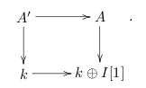
That’s the derived point-of-view on square-zero extensions—the extension map ![{A \rightarrow I[1]}](http://s0.wp.com/latex.php?latex=%7BA+%5Crightarrow+I%5B1%5D%7D&bg=ffffff&fg=000000&s=0 "{A \rightarrow I[1]}") is (or rather, acquires the structure of) a derivation, and that leads to a map is (or rather, acquires the structure of) a derivation, and that leads to a map ![{A \rightarrow k \oplus I[1]}](http://s0.wp.com/latex.php?latex=%7BA+%5Crightarrow+k+%5Coplus+I%5B1%5D%7D&bg=ffffff&fg=000000&s=0 "{A \rightarrow k \oplus I[1]}") . (This can be written down explicitly with cdgas.) . (This can be written down explicitly with cdgas.)
By the cohesiveness axiom, this leads to a homotopy cartesian square of spaces,
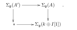
In particular, given a point in )}") , it can be lifted to , it can be lifted to }") if and only if it maps to the basepoint in in if and only if it maps to the basepoint in in ![{\pi_0 \Sigma_{\mathfrak{g}}( k \oplus I[1]) = H_{-2}( \mathfrak{g}) \otimes_k I}](http://s0.wp.com/latex.php?latex=%7B%5Cpi_0+%5CSigma_%7B%5Cmathfrak%7Bg%7D%7D%28+k+%5Coplus+I%5B1%5D%29+%3D+H_%7B-2%7D%28+%5Cmathfrak%7Bg%7D%29+%5Cotimes_k+I%7D&bg=ffffff&fg=000000&s=0 "{\pi_0 \Sigma_{\mathfrak{g}}( k \oplus I[1]) = H_{-2}( \mathfrak{g}) \otimes_k I}") . (Moreover, the set of lifts is a torsor over . (Moreover, the set of lifts is a torsor over  \otimes_k I}") .) .)
In this way, it follows that there is always a canonical tangent-obstruction theory derived directly from the DGLA, and the obstruction theory can be interpreted simply in terms of the long exact sequence of a fibration. The naturality of the obstruction theory (which can be observed classically, without DGLAs) has many useful applications.
Example 4: In the problem of lifting a deformation from ![\mathrm{Spec} k[\epsilon]/\epsilon^2](http://s0.wp.com/latex.php?latex=%5Cmathrm%7BSpec%7D+k%5B%5Cepsilon%5D%2F%5Cepsilon%5E2&bg=ffffff&fg=29303b&s=0 "\mathrm{Spec} k[\epsilon]/\epsilon^2") to to ![\mathrm{Spec} k[\epsilon]/\epsilon^3](http://s0.wp.com/latex.php?latex=%5Cmathrm%7BSpec%7D+k%5B%5Cepsilon%5D%2F%5Cepsilon%5E3&bg=ffffff&fg=29303b&s=0 "\mathrm{Spec} k[\epsilon]/\epsilon^3") , we note that the first object is represented by a cycle , we note that the first object is represented by a cycle  in in  —or rather —or rather  . The Maurer-Cartan equation states simply that it is a cycle. But to lift it to a Maurer-Cartan element modulo . The Maurer-Cartan equation states simply that it is a cycle. But to lift it to a Maurer-Cartan element modulo  , the obstruction becomes precisely , the obstruction becomes precisely ![[x, x]](http://s0.wp.com/latex.php?latex=%5Bx%2C+x%5D&bg=ffffff&fg=29303b&s=0 "[x, x]") . .
2. Hilb and Pic
(I learned this from Mumford’s Lectures on curves on an algebraic surface.)
Let be a smooth, projective surface over the algebraically closed field of characteristic zero. A natural object of study is the collection of curves on . This set is not simply a set; it acquires the structure of a scheme. In other words, there is a scheme  which parametrizes curves (or rather, flat families of curves) on . The scheme is a disjoint union of components of the Hilbert scheme . which parametrizes curves (or rather, flat families of curves) on . The scheme is a disjoint union of components of the Hilbert scheme .
Let’s say we are trying to construct families of curves on . Given a curve  , the tangent space to at is given by , the tangent space to at is given by
,")
as one would expect: a field of normal vectors should give an infinitesimal way to wiggle . One can prove this (i.e., compute the tangent space to ) by using the moduli interpretation, and by studying flat families of curves over ![{\mathrm{Spec} k[\epsilon]/\epsilon^2}](http://s0.wp.com/latex.php?latex=%7B%5Cmathrm%7BSpec%7D+k%5B%5Cepsilon%5D%2F%5Cepsilon%5E2%7D&bg=ffffff&fg=000000&s=0 "{\mathrm{Spec} k[\epsilon]/\epsilon^2}") . .
More generally, the DGLA for the deformation problem “imbedded deformations of in ” is given by (derived) global sections of the sheaf of DGLAs which is the homotopy fiber of the map
|_C,")
that is, the normal sheaf shifted by : ![{\mathcal{N}_C[-1]}](http://s0.wp.com/latex.php?latex=%7B%5Cmathcal%7BN%7D_C%5B-1%5D%7D&bg=ffffff&fg=000000&s=0 "{\mathcal{N}_C[-1]}") . .
In other words, we expect to construct a }") -dimensional family of deformations of . However, we can’t necessarily do this, because is not necessarily smooth at . What we’ve just done is compute the embedding dimension (dimension of the Zariski tangent space), while we want the Krull dimension. To do this, we’ll need to study higher order deformations and obstructions, and for this we’ll need a bit more about the global geometry of . -dimensional family of deformations of . However, we can’t necessarily do this, because is not necessarily smooth at . What we’ve just done is compute the embedding dimension (dimension of the Zariski tangent space), while we want the Krull dimension. To do this, we’ll need to study higher order deformations and obstructions, and for this we’ll need a bit more about the global geometry of .
3. The map to the Picard scheme
Let’s keep the notation of the previous section. There are many curves on , but there is also an equivalence relation one can impose on them: linear equivalence. Curves may move in -families, and we can break the problem of studying curves on into two pieces: studying the various families and studying the equivalence classes. Let’s see this in the following example of a criterion for smoothness of .
In more sophisticated terms, one has a morphism

sending a curve to the line bundle }") . In order to understand , one wants to understand the base and the fibers. . In order to understand , one wants to understand the base and the fibers.
- The fiber of over a line bundle
 consists of all curves in the linear equivalence class : that is, the projective space consists of all curves in the linear equivalence class : that is, the projective space ^{\vee}) }") . So, understanding the fibers of is a question of computing some dimensions, which we can try to get at via Riemann-Roch type formulas. . So, understanding the fibers of is a question of computing some dimensions, which we can try to get at via Riemann-Roch type formulas.
- The target
 is a proper group scheme, and since the characteristic is zero, it is smooth (hence an abelian variety). is a proper group scheme, and since the characteristic is zero, it is smooth (hence an abelian variety).
If is a smooth curve, then the normal bundle on is given by /\mathcal{O}}") , so that we have an exact sequence , so that we have an exact sequence
 \rightarrow \mathcal{N}_C \rightarrow 0.")
Theorem (Severi-Kodaira-Spencer) Let be a curve such that the map ) \rightarrow H^1( C, \mathcal{N}_C)}") is zero. Then is smooth at . is zero. Then is smooth at .
Proof sketch: There is a canonical obstruction theory for deformations of in , given by }") . Similarly, there is a canonical obstruction theory for deformations of line bundles on , given by . Similarly, there is a canonical obstruction theory for deformations of line bundles on , given by }") . The DGLA associated to this problem is given by . The DGLA associated to this problem is given by /k}") . .
The map of deformation problems  induces (say via DGLA theory) a map of obstruction theories that one can identify as coming from the coboundary map induces (say via DGLA theory) a map of obstruction theories that one can identify as coming from the coboundary map
) \rightarrow H^2( X, \mathcal{O}_X).")
By hypothesis, this map is injective.
Therefore, to show that the obstructions to deforming in vanish, it suffices to show that the obstructions vanish in }") . But the obstructions there vanish because is smooth and there are no obstructions to deforming a line bundle. . But the obstructions there vanish because is smooth and there are no obstructions to deforming a line bundle.
Filed under: algebraic geometry, topology Tagged: deformation theory, DGLAs, obstruction theory  | | Wednesday, May 22nd, 2013 | | LJ.Rossia.org makes no claim to the content supplied through this journal account. Articles are retrieved via a public feed supplied by the site for this purpose. |
| 6:51 pm |
Hyperelliptic and trigonal curves Let be a genus curve over the field of complex numbers. I’ve been trying to understand a little about special linear series on : that is, low degree maps , or equivalently divisors on that move in a pencil. Once the degree is at least  , any divisor will produce a map to (in fact, many maps), and these fit into nice families. In degrees , any divisor will produce a map to (in fact, many maps), and these fit into nice families. In degrees  , maps are harder to write down, and the families they form (for fixed , maps are harder to write down, and the families they form (for fixed  ) aren’t quite as nice. ) aren’t quite as nice.
However, it turns out that there are varieties of special linear series—that is, varieties parametrizing line bundles of degree with a certain number of sections, and techniques from deformation theory and intersection theory can be used to bound below and predict their dimensions (the predictions will turn out to be accurate for a general curve). For instance, one can show that any genus curve has a map to of degree at most  , but for degrees below that, the “general” genus curve does not admit such a map. This is the subject of the Brill-Noether theory. , but for degrees below that, the “general” genus curve does not admit such a map. This is the subject of the Brill-Noether theory.
In this post, I’d just like to do a couple of low-degree examples, to warm up for more general results. Most of this material is from Arbarello-Cornalba-Griffiths-Harris’s book Geometry of algebraic curves.
1. Hyperelliptic curves
For  , we are considering hyperelliptic curves: that is, curves with a degree two map to . An application of the Riemann-Hurwitz formula shows that the hyperelliptic map , we are considering hyperelliptic curves: that is, curves with a degree two map to . An application of the Riemann-Hurwitz formula shows that the hyperelliptic map
must be branched over exactly  points. In other words, it is a two-sheeted cover of , and the sheets come together at points. Since it is a degree two cover, it is necessarily Galois, and has a hyperelliptic involution points. In other words, it is a two-sheeted cover of , and the sheets come together at points. Since it is a degree two cover, it is necessarily Galois, and has a hyperelliptic involution  over with those branch points as its fixed points, such that over with those branch points as its fixed points, such that
 \stackrel{\phi}{\simeq} \mathbb{P}^1.")
When  , is an elliptic curve (once one chooses an origin on ), and the hyperelliptic involution can be realized as , is an elliptic curve (once one chooses an origin on ), and the hyperelliptic involution can be realized as  with respect to the group law on . The resulting map with respect to the group law on . The resulting map }") can be realized, for a Weierstrass curve can be realized, for a Weierstrass curve  , by the function , by the function  which respects the involution : in analytic terms, the hyperelliptic map is given by the Weierstrass which respects the involution : in analytic terms, the hyperelliptic map is given by the Weierstrass  -function. The ramification points of this map are the fixed points of the involution , or the four 2-torsion points on . -function. The ramification points of this map are the fixed points of the involution , or the four 2-torsion points on .
In this case, it’s important that the hyperelliptic map is not unique (even up to automorphisms of ). Namely, the hyperelliptic map depended upon the choice of an origin , and then was given by the divisor }") —which moved in a “pencil” and thus defined a map to . (In other words, the line bundle —which moved in a “pencil” and thus defined a map to . (In other words, the line bundle }") corresponding to the divisor had a two-dimensional space of sections corresponding to the divisor had a two-dimensional space of sections )}") .) However, a different .) However, a different  would have provided a different line bundle would have provided a different line bundle }") and a different map to , except for three exceptional choices of . and a different map to , except for three exceptional choices of .
However, in genus , the hyperelliptic map on a curve (if it exists) is unique. To see this, we use the following lemma, called the basepoint-free pencil trick.
Lemma 1 Let  be line bundles on a curve . Let be line bundles on a curve . Let  be sections of be sections of }") without common zeros and consider the map without common zeros and consider the map
 \oplus s_2 H^0( \mathcal{M}) \rightarrow H^0( \mathcal{L} \otimes \mathcal{M}) .")
Then the kernel of this map is }") . .
Proof: Indeed, one has an exact sequence of sheaves

where the first map sends a section  of of  to the pair to the pair }") . This is precisely a Koszul-type complex, for the regular sequence . This is precisely a Koszul-type complex, for the regular sequence }") —regularity follows because the vanishing loci are disjoint. Taking global sections gives the desired claim. —regularity follows because the vanishing loci are disjoint. Taking global sections gives the desired claim.
Let’s now suppose that is a hyperelliptic curve of genus  and are two degree two line bundles with and are two degree two line bundles with  ; that means they’re generated by their global sections (since if they had a basepoint, one would get a degree one line bundle with sections). The basepoint-free pencil trick now shows that, if ; that means they’re generated by their global sections (since if they had a basepoint, one would get a degree one line bundle with sections). The basepoint-free pencil trick now shows that, if  , then , then
 \geq 4,")
where  has degree four. Since has degree four. Since  >0}") , we must have , we must have
 = 4,")
since for any line bundle  on a curve of genus on a curve of genus  , we have , we have  \leq \deg \mathcal{N}}") for for  : otherwise we could keep subtracting points of to get a degree one map to . : otherwise we could keep subtracting points of to get a degree one map to .
Now let’s apply the basepoint-free pencil trick to and . We get
 \geq 6,")
and, once again, equality holds since  = 6}") . Inductively, we get . Inductively, we get
 = 2n + 2.")
Taking  , we know that this has to be equal to , we know that this has to be equal to  , so that . , so that .
In other words, the choice of a hyperelliptic map is a condition, not extra data (modulo automorphisms of ). For example, when , the hyperelliptic map can be described as the canonical map: the map associated to the canonical line bundle. To specify a hyperelliptic curve of genus is thus equivalent to specifying points on over which the degree two cover is branched, modulo automorphisms of . In other words, the moduli space of hyperelliptic curves is given by
/ \mathrm{Aut}(\mathbb{P}^1),")
where  is the configuration space of is the configuration space of  distinct (unordered) points of . In particular, the dimension is given by distinct (unordered) points of . In particular, the dimension is given by
 = 2g - 1,")
so that hyperelliptic curves form a rather small subspace of the moduli space of curves, which has dimension  . Moreover, it is a unirational variety: it admits a dominant rational map from a projective space. This is in sharp contrast to the moduli space . Moreover, it is a unirational variety: it admits a dominant rational map from a projective space. This is in sharp contrast to the moduli space  , which is of general type for , which is of general type for  by a celebrated theorem of Harris and Mumford. by a celebrated theorem of Harris and Mumford.
2. Trigonal curves
Let’s consider the next case: that of a degree three map (or a trigonal curve). We will also assume that the genus of is at least .
In other words, there exists a basepoint-free line bundle on of degree three, defining the map . In fact, in this case, we have
 = 2,")
and so the map is associated to a complete linear system. One way to see this is to appeal to Clifford’s theorem, which states that:
Theorem 2 (Clifford) For a line bundle of degree at most  on a curve , one has on a curve , one has
 - 1) \leq \deg \mathcal{L}.")
Observe that  - 1}") is the dimension of the complete linear system associated to , i.e. the projective space is the dimension of the complete linear system associated to , i.e. the projective space }") . In this case, Clifford’s theorem shows that the linear system associated to a degree three line bundle on (if . In this case, Clifford’s theorem shows that the linear system associated to a degree three line bundle on (if  \geq 3}") ) has dimension at most , which was our claim. ) has dimension at most , which was our claim.
Every curve of genus  is either hyperelliptic or trigonal. Given a genus two curve, we already know that it is hyperelliptic via the canonical map. Let’s look at the next two cases. is either hyperelliptic or trigonal. Given a genus two curve, we already know that it is hyperelliptic via the canonical map. Let’s look at the next two cases.
Example 1 Given a genus three curve , if it is not hyperelliptic, the canonical map imbeds as a smooth plane quartic in , and projection from a point on is a degree three map from to .
Example 2 Given a genus four curve, if it is not hyperelliptic, the canonical map  imbeds as the (degree six) complete intersection of a quadric and a cubic in . Let’s admit this, and see how to produce the degree three map . imbeds as the (degree six) complete intersection of a quadric and a cubic in . Let’s admit this, and see how to produce the degree three map .
We need to produce three points on which move in a pencil. The Riemann-Roch theorem, in its “geometric” form, states that this is equivalent to finding  such that the images of such that the images of  via the canonical imbedding live inside a line, a via the canonical imbedding live inside a line, a  . In other words, impose one less than the expected number of linear conditions on differential 1-forms in : we have . In other words, impose one less than the expected number of linear conditions on differential 1-forms in : we have
) = h^0(K) - 2,")
rather than  - 3}") . .
To produce these three points, observe that a quadric always contains a : in fact, lots of copies of . Now take the three points of intersection between and given by Bezout’s theorem; they are in and live on a line, and so move in a pencil. (This is the sort of argument that Brill-Noether theory does very efficiently, in higher genera when one doesn’t have as clear a picture of curves.)
Once again, trigonal divisors on a curve — degree three divisors that move in a pencil without base points — are very special divisors for large , and we should expect them to be in short supply.
Proposition 3 A curve of genus cannot be both hyperelliptic and trigonal.
Proof: To see this, suppose given a degree two map and a degree three map  . Equivalently, suppose given line bundles on of degrees . Equivalently, suppose given line bundles on of degrees  with with  = h^0(\mathcal{M}) = 2}") . .
The basepoint-free pencil trick now implies that
 \geq h^0(\mathcal{M}) + h^0( \mathcal{M}) = 4.")
If the genus is at least four, then is a degree five special divisor (of degree at most ) whose  contradicts Clifford’s theorem. contradicts Clifford’s theorem.
If the genus is four, then the result fails. Namely, we can take a smooth two-dimensional quadric surface (i.e., a  ), and take a smooth divisor of type ), and take a smooth divisor of type }") . Given a smooth curve in of type . Given a smooth curve in of type }") in , the genus is given by in , the genus is given by  (b-1)}") , so if , so if  the genus is four. Such a curve comes with two natural degree three maps to , which must be distinct since the curve is imbedded in . In fact, it follows from this — since every (edit: not quite, some of these live on singular quadrics and are trigonal in only one way) nonhyperelliptic genus four curve is given by a the genus is four. Such a curve comes with two natural degree three maps to , which must be distinct since the curve is imbedded in . In fact, it follows from this — since every (edit: not quite, some of these live on singular quadrics and are trigonal in only one way) nonhyperelliptic genus four curve is given by a }") -curve in — that the general curve of genus four has (at least) two distinct maps . -curve in — that the general curve of genus four has (at least) two distinct maps .
Proposition 4 A curve of genus  cannot be trigonal in two different ways. cannot be trigonal in two different ways.
Proof: Similarly, suppose there exist two different line bundles of degree and with . In this case, we can use the basepoint-free pencil trick (again!) to get
and that contradicts the equality case of Clifford’s theorem: is special and has degree too small to be the canonical divisor.
It’s interesting that this pattern does not persist: a curve (of high genus) can be tetragonal in infinitely many ways. To construct such examples, consider bi-elliptic curves: that is, curves with a degree two map for an elliptic curve. By increasing the branching, we can make of genus as high as we want. Then there are lots of degree four maps

given by using the (many distinct) degree two maps  . .
Filed under: algebraic geometry Tagged: hyperelliptic curves, moduli of curves, trigonal curves  | | Tuesday, April 2nd, 2013 | | LJ.Rossia.org makes no claim to the content supplied through this journal account. Articles are retrieved via a public feed supplied by the site for this purpose. |
| 7:27 pm |
Divest from climate change! I wrote this for a guest post on Cathy O’Neil’s blog mathbabe.
Climate change is one of those issues that I heard about as a kid, and I assumed naturally that scientists, political leaders, and the rest of the world would work together to solve it. Then I grew up and realized that never happened.
Carbon dioxide emissions are continuing to rise and extreme weather is becoming normal. Meanwhile, nobody in politics seems to want to act, even when major scientific organizations — and now the World Bank — have warned us in the strongest possible terms that the current path towards  or more warming is an absolutely terrible idea (the World Bank called it “devastating”). or more warming is an absolutely terrible idea (the World Bank called it “devastating”).
A little frustrated, I decided to show up last fall at my school’s umbrella environmental group to hear about the various programs. Intrigued by a curious-sounding divestment campaign, I decided to show up at the first meeting. I had zero knowledge of or experience with the climate movement, and did not realize what it was going to become.
Divestment from fossil fuel companies is a simple and brilliant idea, popularized by Bill McKibben’s article “Global Warming’s Terrifying New Math.” As McKibben observes, there are numerous reasons to divest, both ethical and economic. The fossil fuel reserves of these companies — a determinant of their market value — are five(!) times what scientists estimate can be burned to stay within 2 degree warming. Investing in fossil fuels is therefore a way of betting on climate change. It’s especially absurd for universities to invest in them, when much of the research on climate change took place there.
The other side of divestment is symbolic. It’s not likely that Congress will be able to pass a cap-and-trade or carbon tax system anytime soon, especially when fossil fuel companies are among the biggest contributors to political campaigns. A series of university divestments would draw attention to the problem. It would send a message to the world: that fossil fuel companies should be shunned, for basing their business model on climate change and then for lying about its dangers. This reason echoes the apartheid divestment campaigns of the 1980s.
With support from McKibben’s organization 350.org, divestment took off last fall to become a real student movement, and today, over 300 American universities have active
divestment campaigns from their students. Four universities — Unity College,
Hampshire College, Sterling College, and College of the Atlantic — have already divested. Divestment is spreading both to Canadian universities and to other non-profit organizations. We’ve been covered in the New York Times, endorsed by Al Gore, and, on the other hand, recently featured in a couple of rants by Fox News.
Divest Harvard
At Harvard, we began our fall semester with a small group of us quietly collecting student petition signatures, mostly by waiting outside the dining halls, but occasionally by going door-to-door among dorms. It wasn’t really clear how many people supported us: we received a mix of enthusiasm, indifference, and occasional amusement from other students.
But after enough time, we made it to 1,000 petition signatures. That was enough to allow us to get a referendum on the student government ballot. The ballot is primarily used to elect student government leaders, but it was our campaign that rediscovered the use of referenda as a tool of student activism. (Following us, two other worthy campaigns — one on responsible investment more generally and one about sexual assault — also created their own referenda.)
After a week of postering and reaching out to student groups, our proposition—that Harvard should divest—won with 72% of the undergraduate student vote. That was a real turning point for us. On the one hand, having people vote on a referendum isn’t the same as engaging in the one-on-one conversations that we did when convincing people to sign our petition. On the other hand, the 72% showed that we had a real majority in support. The statistic was quickly picked up by the media, since we were the first school to win a referendum on divestment (UNC has since had a winning referendum with 77% support).
That was when the campaign took off. People began to take us seriously. The Harvard administration, which had previously said that they had no intention of considering divestment, promised a serious, forty-five minute meeting with us. We didn’t get what we had aimed for — a private meeting with President Drew Faust — but we had acquired legitimacy from the administration. We were hopeful that we might be able to negotiate a compromise, and ended our campaign last fall satisfied, plotting the trajectory of our campaign at our final meeting.

The spring semester started with a flurry of additional activity and new challenges. On the one hand, we had to plan for the meeting with the administration—more precisely, the Corporation Committee on Social Responsibility. (The CCSR is the subgroup of the Harvard Corporation that decides on issues such as divestment.) But we also knew that the fight couldn’t be won solely within the system. We had to work on building support on campus, from students and faculty, with rallies and speakers; we also had to reach out to alumni and let them know about our campaign. Fortunately, the publicity generated last semester had brought in a larger group of committed students, and we were able to split our organization into working groups to handle the greater responsibilities.
In Februrary, we got our promised meeting with three members the administration. With three representatives from our group meeting with the CCSR, we had a rally with about 40 people outside to show support:

In the meeting, the administration representatives reiterated their concern about climate change, but questioned divestment as a tool. Unfortunately, since the meeting, they have continued to reiterate their “presumption against divestment” (a phrase they have used with previous movements). This is the debate we—and students across the nation—are going to have to win. Divestment alone isn’t going to slow the melting of the Arctic, but it’s a powerful tool to draw attention to climate change and force action from our political system—as it did against apartheid in the 1980s. There isn’t much time left.
One of the most inspirational things I’ve heard this semester was at the Forward on Climate rally in Washington, D.C. last month, which most of our group attended. Addressing a crowd of 40,000 people, Bill McKibben said “All I ever wanted to see was a movement of people to stop climate change, and now I’ve seen it.” To me, that’s one of the exciting and hopeful aspects about divestment—that it’s a movement of the people. It’s fundamentally an issue of social justice that we’re facing, and our group’s challenge is to convince Harvard to take it seriously enough to stand up against the fossil fuel industry.
In the meantime, our campaign has been trying to build support from student groups, alumni, and faculty. In a surprise turnaround, one of our members convinced alumnus Al Gore to declare his support for the divestment movement at a recent event on campus. We organized a teach-in the Tuesday before last featuring writer and sociologist Juliet Schor. On April 11, we will be holding
a large rally outside Massachusetts Hall to close out the year and to show support for divestment; we’ll be presenting our petition signatures to the administration.
Here’s our most recent picture, taken for the National Day of Action, with some supportive friends from the chess club:

Thanks to Joseph Lanzillo for proofreading a draft of this post.
Filed under: climate change Tagged: Bill McKibben, climate change, Divest Harvard, fossil fuel divestment  | | Saturday, April 20th, 2013 | | LJ.Rossia.org makes no claim to the content supplied through this journal account. Articles are retrieved via a public feed supplied by the site for this purpose. |
| 12:39 am |
Some updates It’s been a busy semester, and I haven’t done a great job of updating this blog lately. I have a couple of posts in preparation, but in the meantime:
- I gave a talk on the nilpotence and periodicity theorems in stable homotopy theory at the pre-Talbot seminar (a.k.a. Juvitop) at MIT. All the talks this semester were videotaped; the video of mine is here. The results are really beautiful, showing that the “global” picture of stable homotopy theory exactly parallels the geometry of the moduli stack of formal groups.
- I’ve been taking notes from a course of Joe Harris on the representation theory of Lie groups. Unfortunately, I’m unable to include the many pictures that were drawn in lectures, and the notes are somewhat incomplete.
- I’m spending the summer at the REU program at Emory, and I’ll be thinking about problems in moduli of curves. It should be interesting to get a little experience with algebraic geometry. In particular, I’m going to try to focus this blog in that direction over the next couple of months.
Filed under: Uncategorized Tagged: nilpotence theorem  | | Sunday, April 21st, 2013 | | LJ.Rossia.org makes no claim to the content supplied through this journal account. Articles are retrieved via a public feed supplied by the site for this purpose. |
| 2:04 am |
Deformation theory and DGLAs I There’s a “philosophy” in deformation theory that deformation problems in characteristic zero come from dg-Lie algebras. I’ve been trying to learn a little about this. Precise statements have been given by Lurie and Pridham which consider categories of “derived” deformation problems (i.e., deformation problems that can be evaluated on derived rings) and establish equivalences between them and suitable (higher) categories of dg-Lie algebras. I’ve been reading in particular Lurie’s very enjoyable survey of his approach to the problem, which sketches the equivalence in an abstract categorical context with the essential input arising from Koszul duality between Lie algebras and commutative algebras. In this post, I’d just like to say what a “deformation problem” is in the derived world.
1. Introduction
Let  be a classical moduli problem. Abstractly, we will think of as a functor be a classical moduli problem. Abstractly, we will think of as a functor

such that, for a (commutative) ring , the set }") will be realized as maps from into a geometric object—a scheme or maybe an algebraic space. will be realized as maps from into a geometric object—a scheme or maybe an algebraic space.
Example 1 could be the functor that sends to the set of closed subschemes of  which are flat over . In this case, comes from a scheme: the Hilbert scheme. which are flat over . In this case, comes from a scheme: the Hilbert scheme.
We want to think of as some kind of geometric object and, given a point  for a field (that is, an element of for a field (that is, an element of }") ), we’d like to study the local structure of near ), we’d like to study the local structure of near  . .
Grothendieck’s idea is that we can do this by studying maps from small schemes into . Namely, let  be the category of artinian -algebras with residue field ; then for be the category of artinian -algebras with residue field ; then for  , is a “nilthickening” of , is a “nilthickening” of  . We study maps . We study maps  which agree with on which agree with on  . That is, we study diagrams . That is, we study diagrams

which we can think of small deformations of the point .
If is a scheme, then understanding all these maps amounts to understanding the formal completion of at the point . Even otherwise, a combination of tools such as Grothendieck’s formal GAGA and Artin’s approximation theorem can enable one to go from such “formal deformations” to global deformations (over schemes much bigger than a fuzzy point).
Let’s axiomatize this:
Definition 1 A deformation functor is a functor  satisfying certain axioms: satisfying certain axioms:
 = \ast}") . (This is the “formal” part of the definition.) . (This is the “formal” part of the definition.)- Given a diagram in ,
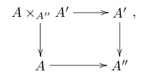 where the maps where the maps  are surjective, the diagram are surjective, the diagram
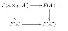
is a pull-back square of sets.
The second condition is a reflection of the fact that  }") is the push-out in the category of schemes, is the push-out in the category of schemes,  . .
Example 2 Given a scheme and a point  , we define a functor , we define a functor  on by sending to the set of maps on by sending to the set of maps  that restrict to on the “closed point.” This is a deformation functor, called the formal completion of at . The name is because that restrict to on the “closed point.” This is a deformation functor, called the formal completion of at . The name is because
 = \hom_k( \widehat{\mathcal{O}_{X, x}}, R),")
so that the deformation functor is prorepresentable—it’s realized by maps out of a complete local ring.
Example 3 As a result, the deformation problem of closed subschemes in  is always prorepresentable. That is, given a closed subscheme is always prorepresentable. That is, given a closed subscheme  , we can look at small deformations of : that is, flat subschemes of that are “thickenings” of (restrict to on the closed fiber). This deformation problem is prorepresentable because of the representability of the Hilbert scheme. However, it’s possible to see this directly, using Schlessinger’s criterion; the deformation problem for closed subschemes of can be studied “directly” and behaves well. Given this well-behaved deformation theory, a deep representability theorem of Artin can be used to show that the Hilbert scheme exists (at least as an algebraic space). As I understand, this sort of argument is very important in the derived context. , we can look at small deformations of : that is, flat subschemes of that are “thickenings” of (restrict to on the closed fiber). This deformation problem is prorepresentable because of the representability of the Hilbert scheme. However, it’s possible to see this directly, using Schlessinger’s criterion; the deformation problem for closed subschemes of can be studied “directly” and behaves well. Given this well-behaved deformation theory, a deep representability theorem of Artin can be used to show that the Hilbert scheme exists (at least as an algebraic space). As I understand, this sort of argument is very important in the derived context.
As time went on, people realized that it’s of interest to replace “sets” by “groupoids” in the definition of a moduli problem. Rather than do that, let’s take the plunge to the derived world.
2. The principal actors
Let be a field of characteristic zero.
Definition 2
- We let
 be the category (throughout, be the category (throughout, }") -category) of connective -algebras over . This is the replacement for “commutative rings.” Since is characteristic zero, -algebras may be modeled by commutative differential graded -algebras. -category) of connective -algebras over . This is the replacement for “commutative rings.” Since is characteristic zero, -algebras may be modeled by commutative differential graded -algebras.
- Let
 be the full subcategory of consisting of -algebras such that: be the full subcategory of consisting of -algebras such that:
 for for  . .- Each homotopy group
 is a finite-dimensional vector space over . is a finite-dimensional vector space over .
 is artinian with residue field . is artinian with residue field .
This is the replacement for the category ; now we’re allowing a small amount of “homotopy fuzz.” Given any object  , there is a canonical augmentation map (well defined up to a contractible space) , there is a canonical augmentation map (well defined up to a contractible space)  . .
Let  be the category of spaces. be the category of spaces.
Definition 3 A formal moduli problem is a functor

such that:
 }") is contractible. is contractible.- Let
 and suppose given maps both of which induce surjections on and suppose given maps both of which induce surjections on  . Then the natural map . Then the natural map
 \rightarrow F(A) \times_{F(A')} F(A'')")
is a homotopy equivalence.
There is a natural category  of formal moduli problems, where the morphisms are the natural transformations. of formal moduli problems, where the morphisms are the natural transformations.
In this definition, the first condition is the reason for the word “formal.” For example, given a moduli problem, meaning a functor  , and a point , and a point }") , we can define the formal completion of at via , we can define the formal completion of at via
 = \mathrm{fib}( \mathcal{M}(A) \rightarrow \mathcal{M}(k)),")
where the (homotopy) fiber is taken over the point . This construction is not necessarily a formal moduli problem, since it does not have to satisfy the second condition.
However, the second condition is often satisfied for the following reason: given maps inducing surjections on , then you should think of }") as obtained by “gluing” as obtained by “gluing”  and and  along the common closed subscheme along the common closed subscheme  . Here is an example of this phenomenon. . Here is an example of this phenomenon.
Theorem 4 (DAG IX) Let  be connective -rings with maps inducing surjections on . Let be connective -rings with maps inducing surjections on . Let  denote the category of connective -modules. Then we have an equivalence of categories denote the category of connective -modules. Then we have an equivalence of categories

where the functor sends a connective  -module to the tuple -module to the tuple  }") where where  is the natural equivalence. is the natural equivalence.
In other words, to give a connective module over is the same as giving a module over , a module over  , together with an isomorphism of their base-changes to , together with an isomorphism of their base-changes to  . .
Proof: The functor defined in the statement of the theorem is a colimit-preserving functor, and in fact a left adjoint: the right adjoint  is given by sending a tuple is given by sending a tuple }") to the fiber product in the diagram: to the fiber product in the diagram:
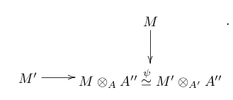
Since tensoring preserves finite limits of modules, it follows that for any -module (not necessarily connective!), it can be recovered from its base-changes to via the above pull-back. In other words,

which states that is a colocalization: it is fully faithful. To show that is an equivalence (on connective modules), it suffices that never annihilates a nontrivial object in  . Suppose given such an object such that the pull-back that one gets is zero. This means that . Suppose given such an object such that the pull-back that one gets is zero. This means that

Choose the smallest index where the homotopy groups don’t vanish, say . Then one has:

Each of the vertical maps are surjective — this can’t happen for a direct sum unless everything vanishes.
For nonconnective modules, the result fails. An example is given by taking ![A = A' = k[x], A'' = k](http://s0.wp.com/latex.php?latex=A+%3D+A%27+%3D+k%5Bx%5D%2C+A%27%27+%3D+k&bg=ffffff&fg=29303b&s=0 "A = A' = k[x], A'' = k") (as discrete (as discrete  -algebras), and with -algebras), and with ![M = \bigoplus_{i \mathrm{\ even}} k[i]](http://s0.wp.com/latex.php?latex=M+%3D+%5Cbigoplus_%7Bi+%5Cmathrm%7B%5C+even%7D%7D+k%5Bi%5D&bg=ffffff&fg=29303b&s=0 "M = \bigoplus_{i \mathrm{\ even}} k[i]") and and ![M' = \bigoplus_{i \ \mathrm{odd} } k[i]](http://s0.wp.com/latex.php?latex=M%27+%3D+%5Cbigoplus_%7Bi+%5C+%5Cmathrm%7Bodd%7D+%7D+k%5Bi%5D&bg=ffffff&fg=29303b&s=0 "M' = \bigoplus_{i \ \mathrm{odd} } k[i]") . .
3. The main result
The main result of DAG X is given by:
Theorem: There is an equivalence of  -categories between -categories between  and the -category of DGLAs (defined by localizing the ordinary category at the quasi-isomorphisms). and the -category of DGLAs (defined by localizing the ordinary category at the quasi-isomorphisms).
In the next couple of posts, I’d like to sketch the proof of this result, which gives a concrete construction of a formal moduli problem out of a DGLA.
Filed under: algebraic geometry Tagged: deformation theory, derived algebraic geometry, DGLAs, formal moduli problems  | | LJ.Rossia.org makes no claim to the content supplied through this journal account. Articles are retrieved via a public feed supplied by the site for this purpose. |
| 8:47 pm |
Deformation theory and DGLAs II Let be a field of characteristic zero. In the previous post, we introduced the category (i.e., -category)  of formal moduli problems over . A formal moduli problem over is a moduli problem, taking values in spaces, that can be evaluated on the class of “derived” artinian -algebras with residue field : this was the category introduced in the previous post. of formal moduli problems over . A formal moduli problem over is a moduli problem, taking values in spaces, that can be evaluated on the class of “derived” artinian -algebras with residue field : this was the category introduced in the previous post.
In other words, a formal moduli problem was a functor
,")
which was required to send itself to a point, and satisfy a certain cohesiveness condition: respects certain pullbacks in (which corresponded geometrically to pushouts of schemes).
The main goal of the series of posts was to sketch a proof of (and define everything in) the following result:
Theorem 7 (Lurie; Pridham) There is an equivalence of categories between and the -category  of DGLAs over . of DGLAs over .
4. Overview
Here’s a rough sketch of the idea. Given a formal moduli problem , we should think of as something like a small space, concentrated at a point but with lots of “infinitesimal” thickening. (Something like a  .) Moreover, has a canonical basepoint corresponding to the “trivial deformation.” That is, we can think of as taking values in pointed spaces rather than spaces. .) Moreover, has a canonical basepoint corresponding to the “trivial deformation.” That is, we can think of as taking values in pointed spaces rather than spaces.
It follows that we can form the loop space  of , which is a new formal moduli problem. However, of , which is a new formal moduli problem. However,  has more structure: it’s a group object in the category of formal moduli problems — that is, it’s some sort of derived formal Lie group. Moreover, knowledge of the original is equivalent to knowledge of together with its group structure: we can recover as has more structure: it’s a group object in the category of formal moduli problems — that is, it’s some sort of derived formal Lie group. Moreover, knowledge of the original is equivalent to knowledge of together with its group structure: we can recover as  (modulo connectivity issues that end up not being a problem). This relation between ordinary objects and group objects (via (modulo connectivity issues that end up not being a problem). This relation between ordinary objects and group objects (via  ) is something very specific to the derived or homotopy world, and it’s what leads to phenomena such as Koszul duality. ) is something very specific to the derived or homotopy world, and it’s what leads to phenomena such as Koszul duality.
In characteristic zero, there is a classical equivalence between formal groups and Lie algebras, given by taking the tangent space at the identity. In the derived world, something like this still works: the (appropriately defined) tangent space to acquires the structure of a DGLA, and this is enough to determine with the group structure. In other words, we have a functor
![\displaystyle \Psi: \mathrm{Moduli}_k \rightarrow \mathrm{dgLie}, \quad \Psi(F) = T( \Omega F) = TF[-1],](http://s0.wp.com/latex.php?latex=%5Cdisplaystyle+%5CPsi%3A+%5Cmathrm%7BModuli%7D_k+%5Crightarrow+%5Cmathrm%7BdgLie%7D%2C+%5Cquad+%5CPsi%28F%29+%3D+T%28+%5COmega+F%29+%3D+TF%5B-1%5D%2C+&bg=ffffff&fg=000000&s=0 "\displaystyle \Psi: \mathrm{Moduli}_k \rightarrow \mathrm{dgLie}, \quad \Psi(F) = T( \Omega F) = TF[-1],")
which implements the equivalence of categories.
Example 4 Given an ordinary -scheme and a -valued point , the formal completion  at is a formal moduli problem; the associated DGLA is the shift at is a formal moduli problem; the associated DGLA is the shift ![{T_x X[-1]}](http://s0.wp.com/latex.php?latex=%7BT_x+X%5B-1%5D%7D&bg=ffffff&fg=000000&s=0 "{T_x X[-1]}") . Here . Here  has to be interpreted in the derived sense. In other words, it’s has to be interpreted in the derived sense. In other words, it’s }") where where  is the cotangent complex. But when is smooth, is concentrated in degree zero (it’s the ordinary tangent bundle) and the associated DGLA is concentrated in degree . is the cotangent complex. But when is smooth, is concentrated in degree zero (it’s the ordinary tangent bundle) and the associated DGLA is concentrated in degree .
In general, the formal completions of ordinary schemes (or Deligne-Mumford stacks, or even derived schemes) always give DGLAs concentrated in strictly negative degrees. These have the property that the associated formal moduli problem, when evaluated on ordinary (discrete) artinian rings, gives discrete sets, as opposed to groupoids or fancier things—there are no infinitesimal automorphisms of the moduli problem when evaluated on ordinary rings. However, these moduli problems still give nontrivial spaces when evaluated on derived artinian rings such as ![{k \oplus k[1]}](http://s0.wp.com/latex.php?latex=%7Bk+%5Coplus+k%5B1%5D%7D&bg=ffffff&fg=000000&s=0 "{k \oplus k[1]}") . .
Example 5 Let be an algebraic group over the algebraically closed field . In this case, the formal completion of  at the trivial torsor corresponds to the DGLA which is the ordinary Lie algebra of , concentrated in degree zero. Here, there are infinitesimal automorphisms, even when evaluated on ordinary rings: the tangent complex (which is the desuspension of the DGLA) is concentrated in degrees at the trivial torsor corresponds to the DGLA which is the ordinary Lie algebra of , concentrated in degree zero. Here, there are infinitesimal automorphisms, even when evaluated on ordinary rings: the tangent complex (which is the desuspension of the DGLA) is concentrated in degrees ![{(-\infty, 1]}](http://s0.wp.com/latex.php?latex=%7B%28-%5Cinfty%2C+1%5D%7D&bg=ffffff&fg=000000&s=0 "{(-\infty, 1]}") . .
Example 6 The formal moduli problems associated to DGLAs concentrated in degrees }") are very different. By Quillen’s rational homotopy theory, such objects correspond precisely to simply connected rational spaces, and should correspond to moduli problems that are somehow “all stacky.” In particular, their tangent space is a coconnective spectrum. are very different. By Quillen’s rational homotopy theory, such objects correspond precisely to simply connected rational spaces, and should correspond to moduli problems that are somehow “all stacky.” In particular, their tangent space is a coconnective spectrum.
As an example, let’s consider a commutative algebraic group, say  . Then one can form . Then one can form  as some sort of higher stack. For an affine scheme as some sort of higher stack. For an affine scheme  , the space of maps , the space of maps  is exactly the space is exactly the space  . In other words, the moduli problem comes from the nonconnective -ring . In other words, the moduli problem comes from the nonconnective -ring ![{\mathbb{Q}[x_{-2}]}](http://s0.wp.com/latex.php?latex=%7B%5Cmathbb%7BQ%7D%5Bx_%7B-2%7D%5D%7D&bg=ffffff&fg=000000&s=0 "{\mathbb{Q}[x_{-2}]}") , where , where  is a free variable in degree is a free variable in degree  . The associated space in rational homotopy theory is . The associated space in rational homotopy theory is }") . .
The associated formal completion sends an to  , where , where  is the “maximal ideal”—the fiber of the augmentation. The associated DGLA is the Lie algebra of homotopy groups of a , shifted by one—so is the “maximal ideal”—the fiber of the augmentation. The associated DGLA is the Lie algebra of homotopy groups of a , shifted by one—so  in degree and zero everywhere else. in degree and zero everywhere else.
5. Construction
In DAG X, Lurie uses various Koszul duality functors to write down the equivalence in question. It’s also possible (and more classical) to describe fairly explicitly the formal moduli problem associated to a DGLA in terms of solutions to the Maurer-Cartan equation.
Let be a DGLA over the field of characteristic zero. In the paper “DG coalgebras as formal stacks,” Hinich explicitly writes down a (formal moduli) functor

In fact, Hinich does so at the level of ordinary categories itself.
Let  be the ordinary category of nonnegatively graded commutative dg-algebras (with homological grading conventions; the differential has degree ), whose total dimension is finite and such that be the ordinary category of nonnegatively graded commutative dg-algebras (with homological grading conventions; the differential has degree ), whose total dimension is finite and such that  is local artinian with residue field . Observe that these are not cofibrant in the usual model structure on cdgas. Let is local artinian with residue field . Observe that these are not cofibrant in the usual model structure on cdgas. Let  be the ordinary category of dg-Lie algebras. Hinich writes down a functor be the ordinary category of dg-Lie algebras. Hinich writes down a functor

where  is the (ordinary) category of Kan complexes. The functor has the property that it respects weak equivalences in each variable: that is, quasi-isomorphic (artinian) cdgas and quasi-isomorphic DGLAs map to homotopy equivalent Kan complexes. For each , this defines a functor is the (ordinary) category of Kan complexes. The functor has the property that it respects weak equivalences in each variable: that is, quasi-isomorphic (artinian) cdgas and quasi-isomorphic DGLAs map to homotopy equivalent Kan complexes. For each , this defines a functor

which preserves weak equivalences, and, as we’ll see below, leads to a formal moduli problem in the sense previously described.
Definition 8 Given a DGLA , a Maurer-Cartan element of is an element  such that such that
![\displaystyle dx + \frac{1}{2}[x, x] = 0. \ \ \ \ \ (1)](http://s0.wp.com/latex.php?latex=%5Cdisplaystyle+dx+%2B+%5Cfrac%7B1%7D%7B2%7D%5Bx%2C+x%5D+%3D+0.+%5C+%5C+%5C+%5C+%5C+%281%29&bg=ffffff&fg=000000&s=0 "\displaystyle dx + \frac{1}{2}[x, x] = 0. \ \ \ \ \ (1)")
Definition 9 Given a DGLA , the space }") (the “space of solutions to the Maurer-Cartan equation”) is defined as the simplicial set (the “space of solutions to the Maurer-Cartan equation”) is defined as the simplicial set }") , where , where  is the algebra of polynomial differential forms on is the algebra of polynomial differential forms on  . It turns out to be a Kan complex. . It turns out to be a Kan complex.
The idea is that, given a DGLA and  , we take to be the maximal ideal of . The DGLA is a nilpotent DGLA (at least in some homotopical sense) and we take the space of solutions to the Maurer-Cartan equation, , we take to be the maximal ideal of . The DGLA is a nilpotent DGLA (at least in some homotopical sense) and we take the space of solutions to the Maurer-Cartan equation,  \stackrel{\mathrm{def}}{=}MC( \mathfrak{g} \otimes \mathfrak{m}_A)}") . In other words, we use the pairing . In other words, we use the pairing
 = MC( \mathfrak{g} \otimes \mathfrak{m}_A).")
Note also that the functor }") is what implements rational homotopy theory, for positively graded. is what implements rational homotopy theory, for positively graded.
We need to use two non-obvious facts here:
- The formal localization
![{\mathbf{dgart}[W^{-1}]}](http://s0.wp.com/latex.php?latex=%7B%5Cmathbf%7Bdgart%7D%5BW%5E%7B-1%7D%5D%7D&bg=ffffff&fg=000000&s=0 "{\mathbf{dgart}[W^{-1}]}") (where (where  is the collection of quasi-isomorphisms) is equivalent to . is the collection of quasi-isomorphisms) is equivalent to .
- The formal localization
![{\mathcal{K}an[W^{-1}]}](http://s0.wp.com/latex.php?latex=%7B%5Cmathcal%7BK%7Dan%5BW%5E%7B-1%7D%5D%7D&bg=ffffff&fg=000000&s=0 "{\mathcal{K}an[W^{-1}]}") (where is the collection of homotopy equivalences) is the -category of spaces. (where is the collection of homotopy equivalences) is the -category of spaces.
In particular, the functor  descends (after applying localization) to a functor descends (after applying localization) to a functor  . It clearly sends itself to . It clearly sends itself to  . To see that we get a formal moduli problem, note that clearly preserves 1-categorical fiber products, and therefore (replacing a cartesian square of by one where desired maps are surjective) preserves fiber products in a good derived sense. . To see that we get a formal moduli problem, note that clearly preserves 1-categorical fiber products, and therefore (replacing a cartesian square of by one where desired maps are surjective) preserves fiber products in a good derived sense.
To make this precise, we need to know a little about the properties of this functor , which is really only well-defined for nilpotent DGLAs:
- There is a good model structure on , where the weak equivalences are the quasi-isomorphisms and the fibrations are the surjections. (This is obtained by transfer from the model structure on chain complexes.)
- Given a fibration (resp. acyclic fibration)
 of nilpotent DGLAs, the map of nilpotent DGLAs, the map  \rightarrow MC(\mathfrak{h})}") is a fibration (resp. acyclic fibration). Consequently, the same is true for is a fibration (resp. acyclic fibration). Consequently, the same is true for  \rightarrow MC( \mathfrak{h} \otimes \mathfrak{m}_A)}") (for ) without the nilpotence assumption. (for ) without the nilpotence assumption.
- Even better,
}") is homotopically well-defined — a quasi-isomorphism between DGLAs leads to a homotopy equivalence on is homotopically well-defined — a quasi-isomorphism between DGLAs leads to a homotopy equivalence on }") ‘s. (Apply Ken Brown’s lemma.) ‘s. (Apply Ken Brown’s lemma.)
- Incidentally, given , a Maurer-Cartan element of is exactly a primitive cycle of the cocommutative coalgebra
}") of Chevalley-Eilenberg chains. This leads to the relation with Koszul duality — Lie algebra homology of Chevalley-Eilenberg chains. This leads to the relation with Koszul duality — Lie algebra homology  is what implements it. is what implements it.
Together, these assertions imply that is a well-defined formal moduli problem, and in fact gives a functor

Classically, it was observed that many formal moduli problems arose in this manner.
Filed under: algebraic geometry, topology Tagged: deformation theory, derived algebraic geometry, DGLAs, Maurer-Cartan equation, rational homotopy theory  | | Thursday, March 21st, 2013 | | LJ.Rossia.org makes no claim to the content supplied through this journal account. Articles are retrieved via a public feed supplied by the site for this purpose. |
| 6:55 pm |
Duality for abelian varieties Let be an abelian variety over the algebraically closed field . In the previous post, we studied the Picard scheme , or rather its connected component  at the identity. The main result was that was itself an abelian variety (in particular, smooth) of the same dimension as , which parametrizes precisely the translation-invariant line bundles on . at the identity. The main result was that was itself an abelian variety (in particular, smooth) of the same dimension as , which parametrizes precisely the translation-invariant line bundles on .
We also saw how to construct isogenies between and . Given an ample line bundle on , the map

is an isogeny. Such maps were in fact the basic tool in proving the above result.
The goal of this post is to show that the contravariant functor

from abelian varieties over to abelian varieties over , is a well-behaved duality theory. In particular, any abelian variety is canonically isomorphic to its bidual. (This explains why the double Picard functor on a general variety is the universal abelian variety generated by that variety, the so-called Albanese variety.) In fact, we won’t quite finish the proof in this post, but we will finish the most important step: the computation of the cohomology of the universal line bundle on  . .
Motivated by this, we set the notation:
Definition 11 We write for .
The main reference for this post is Mumford’s Abelian varieties.
10. The Poincaré line bundle and the biduality map
The first step in understanding the biduality of abelian varieties is to understand the universal line bundle on  . By definition, parametrizes line bundles on algebraically equivalent to zero, so there is a universal line bundle . By definition, parametrizes line bundles on algebraically equivalent to zero, so there is a universal line bundle  , called the Poincaré line bundle, on . , called the Poincaré line bundle, on .
The line bundle has the property that is trivialized on  and and  , and as , and as  varies, the various restrictions of to varies, the various restrictions of to  range exactly over the line bundles on algebraically equivalent to zero: this is precisely the definition of . range exactly over the line bundles on algebraically equivalent to zero: this is precisely the definition of .
As we’ve observed before, there is quite a bit of symmetry in this. Instead of regarding as a family of line bundles on , parametrized by , we can regard it as a family of line bundles on the dual parametrized by . The result is that we get a canonical biduality map

classifying the Poincaré bundle. This is a pointed map, hence a morphism of abelian varieties. The main goal of this post and the next is to show:
Theorem 12 For any abelian variety , the biduality map  is an isomorphism. is an isomorphism.
In particular, this implies a non-obvious fact about the Poincaré bundle : as one restricts to the various fibers  (for (for  ), one gets every translation-invariant line bundle on exactly once. ), one gets every translation-invariant line bundle on exactly once.
The strategy in proving the above theorem is to show first that the biduality map is finite, by a diagram chase and the isogenies  constructed before. Next, we’ll show that the Poincaré bundle isn’t “redundant” on either factor by showing that its Euler characteristic is constructed before. Next, we’ll show that the Poincaré bundle isn’t “redundant” on either factor by showing that its Euler characteristic is ^{\dim X}}") : this will imply that the biduality map is actually an isomorphism. : this will imply that the biduality map is actually an isomorphism.
11. Finiteness of the biduality map
The first goal is to show that the biduality map is a finite morphism: that is, it cannot annihilate a nontrivial abelian subvariety . In other words, in terms of the Poincaré bundle, it states that for any , the restricted bundle  is still nontrivial. is still nontrivial.
To see this, observe that is a family of line bundles on : it’s classified by the map

dual to the inclusion  . The claim is that not only is this family nontrivial, but also that it hits every translation-invariant line bundle on . That is, every translation-invariant line bundle on extends to . In other words: . The claim is that not only is this family nontrivial, but also that it hits every translation-invariant line bundle on . That is, every translation-invariant line bundle on extends to . In other words:
Proposition 13 If  is a map of abelian varieties with finite kernel, then is a map of abelian varieties with finite kernel, then  is surjective. is surjective.
Proof: Given an ample line bundle }") , we have a morphism , we have a morphism

which classifies the bundle  \in \mathrm{Pic}(X \times X)}") , for , for  the multiplication. the multiplication.
The restriction  to is still ample, since is finite, and we have a commutative diagram: to is still ample, since is finite, and we have a commutative diagram:
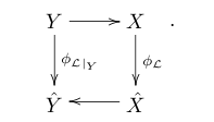
Since  is surjective, it follows that is surjective. is surjective, it follows that is surjective.
This in particular shows that the biduality map must be finite.
12. The cohomology of
Our next goal is to compute the cohomology of the Poincaré bundle on . (In particular, itself is not algebraically equivalent to zero!) We can do this using the Leray spectral sequence and the categorified “orthogonality of characters,” although the argument is a bit technical, and we’ll split it into two sections.
Namely, is a family of line bundles on , parametrized by . By “orthogonality of characters,” each fiber  has vanishing cohomology except when has vanishing cohomology except when  . It follows that the complex . It follows that the complex

which lives in the derived category of sheaves on , is concentrated at the identity  . .
If  is the local ring at , we can localize this complex to get a complex is the local ring at , we can localize this complex to get a complex  of -modules. The general yoga of base-change tells us that is a perfect complex, and the (derived) tensor product of -modules. The general yoga of base-change tells us that is a perfect complex, and the (derived) tensor product  is precisely the cohomology of along the fiber: that is, is precisely the cohomology of along the fiber: that is, }") . .
Let  . Since is concentrated in dimensions . Since is concentrated in dimensions ![{[0, g]}](http://s0.wp.com/latex.php?latex=%7B%5B0%2C+g%5D%7D&bg=ffffff&fg=000000&s=0 "{[0, g]}") , we conclude by Nakayama’s lemma that the cohomology of itself is concentrated in dimensions . Moreover, the cohomology of consists of artinian -modules, because it is supported at the origin. , we conclude by Nakayama’s lemma that the cohomology of itself is concentrated in dimensions . Moreover, the cohomology of consists of artinian -modules, because it is supported at the origin.
That already buys us something. Roughly, there can’t be any cohomology close to zero, because then the derived tensor product with would blow that up into negative dimensions. (The grading is cohomological here.) In fact, we have a precise statement:
Lemma 14 If is a regular local ring of dimension , and is a perfect complex of -modules with artinian cohomology such that the (derived) tensor product is cohomologically concentrated in dimensions  , then has cohomology concentrated in dimensions , then has cohomology concentrated in dimensions  . .
Proof: Induction on . When  and is a field, it is evident. Assume that it is true for regular local rings of dimension and is a field, it is evident. Assume that it is true for regular local rings of dimension  . .
We just have to prove that there is no cohomology below , by Nakayama’s lemma. Given a regular parameter  (in the maximal ideal), we can form (in the maximal ideal), we can form }") , which is a perfect complex of , which is a perfect complex of }") -modules satisfying the same hypotheses. In particular, has no cohomology below dimension by the inductive hypothesis. Now consider the cofiber sequence -modules satisfying the same hypotheses. In particular, has no cohomology below dimension by the inductive hypothesis. Now consider the cofiber sequence
")
and the exact sequence in cohomology
) \rightarrow H^i(P^\bullet) \stackrel{x}{\rightarrow} H^i(P^\bullet).")
For  , this means that multiplication by is injective on , this means that multiplication by is injective on }") ; since these are artinian modules, they must vanish. ; since these are artinian modules, they must vanish.
13. The cohomology of : part 2
Keep the notation of the previous section. Our conclusion is that the derived push-forward  must be supported at the point , and concentrated in cohomological dimension . The claim is that the cohomology in dimension is precisely the ground field . must be supported at the point , and concentrated in cohomological dimension . The claim is that the cohomology in dimension is precisely the ground field .
In fact, we start by noting:
 \otimes_R k = H^g( X, \mathcal{O}_X) = k,")
by Serre duality (recall that  ). It follows that ). It follows that }") has the property that is generated by one element. Moreover, has the property that is generated by one element. Moreover,
 = H^0( Rp_{2*} \mathcal{P} \otimes_R k) = H^0(X, \mathcal{O}_X) = k.")
To see that is in fact , we will use a bit of local duality theory, as explained in this post. Namely, the statement is that the category of artinian modules over is dual to itself, via the local duality functor
.")
In fact,  is given by the derived maps from is given by the derived maps from  to , up to a cohomological shift. to , up to a cohomological shift.
In our case, the (artinian) module has the property that is generated by one element. That doesn’t mean that  , though (not even that along with , though (not even that along with  =k}") : take : take ![{M = k[x]/x^2}](http://s0.wp.com/latex.php?latex=%7BM+%3D+k%5Bx%5D%2Fx%5E2%7D&bg=ffffff&fg=000000&s=0 "{M = k[x]/x^2}") over over ![{R = k[[x]]}](http://s0.wp.com/latex.php?latex=%7BR+%3D+k%5B%5Bx%5D%5D%7D&bg=ffffff&fg=000000&s=0 "{R = k[[x]]}") ). We need to use an additional feature that can be seen using the local duality. The strategy is going to be to show that ). We need to use an additional feature that can be seen using the local duality. The strategy is going to be to show that  is isomorphic to , because is isomorphic to , because  and because the surjection and because the surjection  can’t be lifted further. can’t be lifted further.
Let be a finite complex of projectives quasi-isomorphic to ![{M[-g]}](http://s0.wp.com/latex.php?latex=%7BM%5B-g%5D%7D&bg=ffffff&fg=000000&s=0 "{M[-g]}") (i.e. a “cofibrant replacement”). We observe that for any artinian -algebra , we have (i.e. a “cofibrant replacement”). We observe that for any artinian -algebra , we have  \simeq H^0( \mathcal{P}|_{X \times \mathrm{Spec} S})}") , which cannot surject onto , which cannot surject onto }") simply because cannot be trivialized beyond simply because cannot be trivialized beyond  . .
That last statement is a consequence of the fact that is the solution to a moduli problem: if  pulled back to a trivial bundle, then by definition it would have to be constant at the origin. pulled back to a trivial bundle, then by definition it would have to be constant at the origin.
Now, we can write
 = H^0(P^\bullet \otimes S) = \hom( \mathbb{D}M, S),")
for the local duality functor from artinian -modules to itself. In fact,
![\displaystyle H^0(P^\bullet \otimes S) = H^0( \mathbb{D} \mathbb{D} M[g] \otimes S) = H^0( \mathbf{RHom}( \mathbb{D} M, S)) = \hom(\mathbb{D}M, S).](http://s0.wp.com/latex.php?latex=%5Cdisplaystyle+H%5E0%28P%5E%5Cbullet+%5Cotimes+S%29+%3D+H%5E0%28+%5Cmathbb%7BD%7D+%5Cmathbb%7BD%7D+M%5Bg%5D+%5Cotimes+S%29+%3D+H%5E0%28+%5Cmathbf%7BRHom%7D%28+%5Cmathbb%7BD%7D+M%2C+S%29%29+%3D+%5Chom%28%5Cmathbb%7BD%7DM%2C+S%29.+&bg=ffffff&fg=000000&s=0 "\displaystyle H^0(P^\bullet \otimes S) = H^0( \mathbb{D} \mathbb{D} M[g] \otimes S) = H^0( \mathbf{RHom}( \mathbb{D} M, S)) = \hom(\mathbb{D}M, S).")
The conclusion on  is that: is that:
 maps to nontrivially. In fact, taking maps to nontrivially. In fact, taking  , we find that , we find that }") is one-dimensional, so is one-dimensional, so  . .- In particular,
 for for  an ideal (containing some power of an ideal (containing some power of }") . .
- However, the map
 cannot be lifted under the map cannot be lifted under the map  for any local artinian -algebra. This proves for any local artinian -algebra. This proves  and and  . .
- Dualizing, we find that
 . .
The conclusion that we get (from this calculation plus the degenerate Leray spectral sequence) is:
Theorem 15 The cohomology of the Poincaré bundle is given by:
 = \begin{cases} 0 & \text{if } i \neq g \\ k & \text{if } i = g \end{cases}.")
Filed under: algebraic geometry Tagged: abelian varieties, local duality, Picard scheme  |
LJ.Rossia.org makes no claim to the content supplied through this journal account. Articles are retrieved via a public feed supplied by the site for this purpose.
|


![{k[\epsilon]/\epsilon^2}](http://s0.wp.com/latex.php?latex=%7Bk%5B%5Cepsilon%5D%2F%5Cepsilon%5E2%7D&bg=ffffff&fg=000000&s=0 "{k[\epsilon]/\epsilon^2}") —are given by
—are given by }") where
where  is the tangent bundle (i.e., vector fields).
}") .
. . Specifically, given a square-zero extension of finite-dimensional local
 of
of  \otimes_k I}") to extending the deformation over the inclusion
to extending the deformation over the inclusion  .
. \otimes_k I}") .
.